Archive

QGIS

Ever wondered how to create multi-line labels in QGIS? The new labeling engine has a “Multiline labels” option but it’s not so obvious how to create a usable labeling attribute. Here is how it works (credits to @nhopton on QGIS forum):

  1. Create a big enough text field (if the data doesn’t contain any yet).
  2. In Layer Properties – Fields, chose a “Text edit” edit widget for the label field.
  3. Enter the multi-line text into the label field. You can do this using Attribute Table or Feature Form.

    A feature form with "Text edit" widget

  4. Activate labeling. You’ll have to tick “Multiline labels” option in Layer Labeling Settings – Advanced – Options. That’s it:

    Simple multi-line label example

A common use case is the wish to show multiple attribute values in a feature’s label. Using Field Calculator, you can combine them into multi-line labels. All you need is to combine the fields with the || operator and add ‘\n’ (newline) wherever there should be a line break:

Field1 || '\n' || Field2

Populating a multi-line label field using Field Calculator

And finally, the result:

Multi-line labels displaying city name and population

The aim of QGIS Processing Framework developed by Polymeris is to provide a generic framework for accessing existing geo-processing functionality of e.g. SAGA, GRASS, Orfeo Toolbox, etc. This should enable users to script their geo-processing work in python console and allow development of a tool to graphically build workflows using VisTrails an “open-source scientific workflow and provenance management system”.

For a first impression, Polymeris has published some screenshots of QGIS with SAGA modules loaded: [1],[2]

This project is big and if it turns out well, QGIS will profit enormously from it. Both scriptable geoprocessing functionality and a graphic workflow builder can improve user experience a lot if they are implemented well. You can follow further development on the project homepage on GitHub.

On Wednesday, Allan Maungu announced MXD2QGS, a converter that exports layers from an Arcmap 10 document into a Quantum GIS project file. The tool is built as an ArcToolbox and can be downloaded from the blog.

I’d be very interested to hear whether this tool works for you.

For everyone working with spatial databases in QGIS there comes a time when “Add PostGIS/SpatiaLite Layer” and “RT Sql Layer” start to be annoying. You always have to retype or copy-paste your SQL queries into the user interface if you need to change the tiniest thing in the layer’s definition.

This is where “Fast SQL Layer” can be a real time saver. Fast SQL Layer is a new plugin for QGIS by Pablo T. Carreira. It basically adds an SQL console for loading layers from PostGIS/SpatiaLite into QGIS. And it even comes with syntax highlighting!

Installation

Fast SQL Layer comes with one dependency: Pygments, which is used for syntax highlighting.

On Ubuntu, all you have to do is install it with apt-get:

sudo apt-get install python-pygments

For Windows with OSGeo4W, @Mike_Toews posted this on gis.stackexchange:

I downloaded and extracted Pygments-1.4.tar.gz, then in an OSGeo4W shell within the Pygments-1.4 directory, type python setup.py build then python setup.py install

Usage

When you activate the plugin in plugin manager, a dock widget will appear which contains the console and some fields for specifying the database connection that should be used. Then, you can simply write your SQL query and load the results with one click.

Fast SQL plugin

In this example, I renamed “gid” to “id”, but you can actually edit the values in the drop down boxes to adjust the column names for id and geometry:

A second layer loaded using Fast SQL plugin

It certainly needs some polishing on the user interface side but I really like it.

In a previous post, I’ve described how to create catchment areas with pgRouting shortest_path() function. The solution described there calculates costs from the starting node (aka vertex) to all other nodes in the network. Depending on the network size, this can take a long time. Especially, if you are only interested in relatively small catchment areas (e.g. 50 km around a node in a network covering 10,000 km) there is a lot of unnecessary calculation going on. This is where you might want to use driving_distance() instead.

Driving_distance() offers a parameter for maximum distance/cost and will stop calculations when the costs exceed this limit. But let’s start at the beginning: installing the necessary functions.

Installation

If you have followed my guide to installing pgRouting, you already have some routing functions installed – but not driving_distance(). Weirdly, the necessary SQL scripts are not shipped with the .zip file available on pgRouting’s download page. You need:

routing_dd.sql
routing_dd_wrappers.sql

Both are available through the project repository at Github. Get them and execute them in your pgRouting-enabled database. Now, you should be ready.

Calculating driving distances

To calculate driving distances, we need a query very similar to shortest_path():

CREATE OR REPLACE FUNCTION driving_distance(
sql text,
source_id integer,
distance float8,
directed boolean,
has_reverse_cost boolean)
RETURNS SETOF path_result

The only new value is “distance”. That’s the maximum distance/cost you want to be contained in the result set. “distance” has to be specified in the same units as the cost attribute (which is specified in the “sql” text parameter).

Note: In my opinion, the name “(driving) distance” is misleading. While you can use distance as a cost attribute, you’re not limited to distances. You can use any cost attribute you like, e.g. travel time, fuel consumption, co2 emissions, …

The actual query for a catchment area of 100 km around node # 2000 looks like this:

SELECT * FROM driving_distance('
      SELECT gid AS id,
          start_id::int4 AS source,
          end_id::int4 AS target,
          shape_leng::float8 AS cost
      FROM network',
      2000,
      100000,
      false,
      false)

Interpreting the result

These are the first lines of the result set:

vertex_id;edge_id;cost
294;7262;97400.433506144
297;7236;98012.620979231
335;1095;96849.456306244
347;7263;93617.693852324
364;7098;93573.849081386
366;2551;92702.443434779
378;7263;91994.328368081

The cost attribute contains the total cost of travel from the starting node to the vertex_id node.
We will only be using vertex_id and cost. The use of edge_id is a mystery to me.

Visualizing the result

The easiest way to visualize driving_distance() results is using RT Sql Layer plugin. We need to join the results of driving_distance() with the table containing node geometries:

SELECT *
   FROM node
   JOIN
   (SELECT * FROM driving_distance('
      SELECT gid AS id,
          start_id::int4 AS source,
          end_id::int4 AS target,
          shape_leng::float8 AS cost
      FROM network',
      2000,
      100000,
      false,
      false)) AS route
   ON
   node.id = route.vertex_id

If you color the nodes based on the cost attribute, it will look something like this:
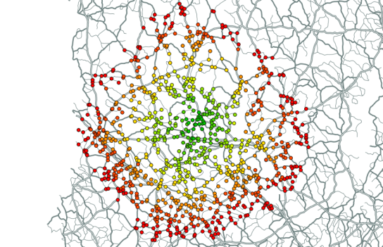
result of pgRouting driving_distance() visualized in QGIS

This year, three QGIS projects made it into Google Summer of Code. Congratulations to all successful students!

These are the accepted OSGEO projects:

QGIS

GRASS

  • GRASS WXGUI WMS service rendering
  • Completion of wxGUI Nviz extension for 3D data visualization in GRASS GIS
  • r.in.modis for GRASS GIS
  • Graphical User Interface for the hydrological tools r.stream* in GRASS GIS

pgRouting

  • Multi-modal public transit routing for pgRouting
  • Time Dependent \ Dynamic Shortest Path Algorithm Implementation for pgRouting

gvSIG

  • Add support to vector data formats for gvSIG Mini
  • Design and implement an API for tiled vectorial support of geo-location data services for gvSIG Mini
    Integration of GGL2 into gvSIG

Opticks

  • Development of a ship detection and classification toolkit for SAR imagery in Opticks
  • Astronomical processing tools for Opticks
  • Photography processing tools for Opticks

Geoserver

  • Enhancing Geoserver Authentication

uDig

  • Catalog View of uDig
  • OSM data mining and editing capabilities in uDig and Geotools

MapServer

  • INSPIRE View Service for MapServer

Others

  • Geoprocessing with Neo4j Spatial
  • PyOSSIM: Python bindings for OSSIM libraries

For a full list including student names check http://www.google-melange.com/gsoc/org/google/gsoc2011/osgeo.

Gistutor.com features a nice tutorial covering raster-based terrain analysis techniques with QGIS and “Raster based terrain analysis” plugin.

Topics covered include: slope analysis, aspect analysis, ruggedness index analysis, total curvature analysis, and shaded relief.

Kudos to Mapperz on gis.stackexchange.com for the pointer.

Analyzing spatio-temporal data using a GIS can be a tedious task without the correct tools. A series of techniques has been developed to visualize spatio-temporal data. These techniques can be divided into two classes: static visualizations and dynamic animations.

In static maps, temporal change can be visualized using appropriate different symbology or annotations. Another option is to create map series with one map for every time frame of interest.

Animated maps are best known from TV weather forecast shows. Animations enable the map user to recognize spatio-temporal relationships more intuitively than static maps could.

Interactive animated maps can help the user to explore and analyze spatio-temporal data. The literature lists the following minimum functionality for interactive animated maps: stop, play, step forward and looping functions. The efficiency of animations can be increased by allowing the user to control the size of visualized time frames and the speed of the animation.

All these functions (and more) have been implemented into Time Manager for QGIS. The user has full control over the animation. Animations can be played forward or backward at any speed. The user can also navigate through the animation step by step or jump to desired points in time using the slider or time input field.

Time Manager dock

Time Manager dock GUI

Besides viewing animations inside QGIS, animations can also also be exported frame-by-frame. These single images can be used as they are or combined into a video file using tools like mencoder.

The connection between spatial objects and the temporal dimension is established using timestamps. A timestamp can consist of either a point in time (e.g. the GPS position of a tracked object at one moment) or a timespan (e.g. a plot of land has been used to grow corn from 2002 to 2005).

Time Manager can handle multiple temporal layers at a time. It’s also possible to specify an offset between layers to achieve different effects. Any vector layer (point, line or polygon) with a correctly formated timestamp attribute can be used. All Time Manager settings are saved into the QGIS project file and are restored when loading an existing project.

According to FOSSGIS presentation feedback the following features are on the most wanted list: support for raster layers and support for year-only timestamps before 19xx.

The plugin installation includes a user manual for quick reference.

Update: For up to date info check Time Manager project page.

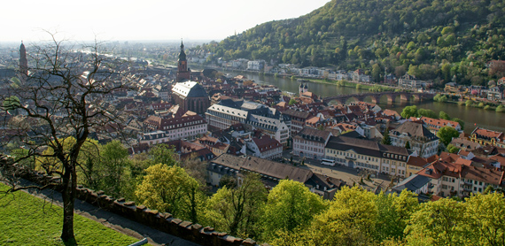
Heidelberg - Home of FOSSGIS2011

FOSSGIS2011 in Heidelberg was a great success for the QGIS project and for me personally. The audience was really impressed by Marco’s and Andreas’ presentation on QGIS Mapserver and GeoExt Web Client. My presentation on Time Manager for QGIS was followed by a series of interesting questions and comments concerning use cases in e.g. land use mapping. Requested features include support for raster layers and support for timestamps before year 19xx.
I’ll be posting an English version of the Time Manager presentation including some additional comments here soon.

QGIS wiki now has it’s own section listing QGIS video tutorials.
If you know of any tutorials not listed yet, leave a comment and I’ll add them.

Together with the newly started “How to I do that in QGIS” tutorial collection, this will hopefully become the number one reference for both new users doing their first GIS-related work and advanced uses interested in the latest QGIS features.