How to create illuminated contours, Tanaka-style

In the category “last night on Twitter”, a challenge I couldn’t resist: creating illuminated contours (aka Tanaka contours) in QGIS. Daniel P. Huffman started the thread by posting this great example:

This was quickly picked up by Hannes Kröger who blogged about his first attempt at reproducing the effect using QGIS and GIMP. Obviously, that left the challenge of finding a QGIS-only solution.

Everything that’s needed to create this effect is a DEM. As Hannes describes in his post, the DEM can then be used to compute the contour lines, e.g. with Raster | Extraction | Contour:

gdal_contour -a ELEV -i 100.0 C:\Users\anita\Geodata\misc\mt-st-helens\10.2.1.1043901.dem C:/Users/anita/Geodata/misc/mt-st-helens/countours

In order to be able to compute the brightness of the illuminated contours, we need to compute the orientation of every subsection of the contours. Therefore, we need to split the contour lines at each node. One way to do this is using v.split from the Processing toolbox:

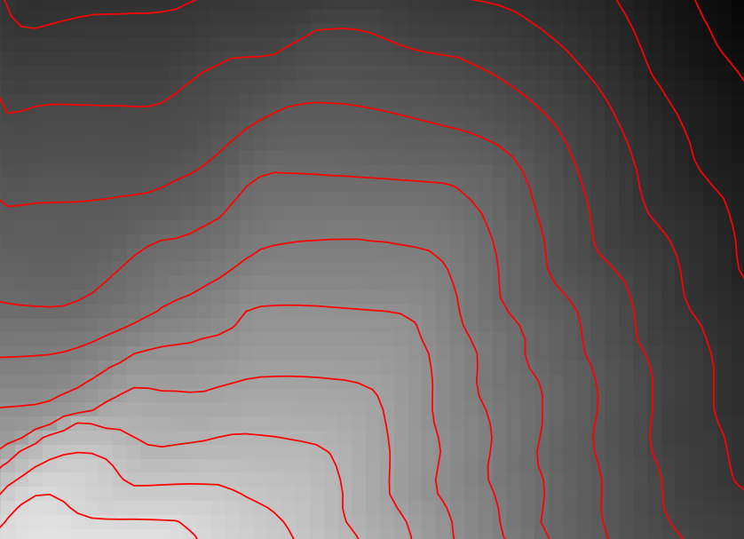
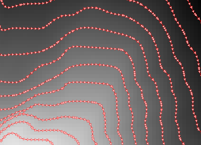
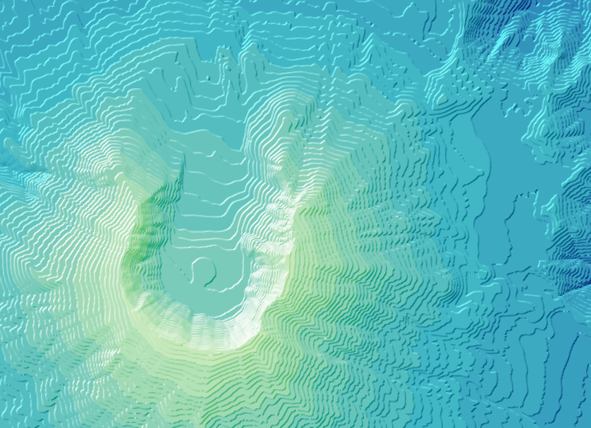
When we split the contours and visualize the result using arrows, we can see that they all wrap around the mountain in clockwise direction (light DEM cells equal higher elevation):

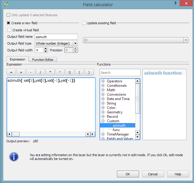
After the split, we can compute the orientation of the contour subsections using, for example, a user-defined function:

"""
Define new functions using @qgsfunction. feature and parent must always be the
last args. Use args=-1 to pass a list of values as arguments
"""

from qgis.core import *
from qgis.gui import *

@qgsfunction(args='auto', group='Custom')
def azimuth(x1,y1,x2,y2, feature, parent):
	p1 = QgsPoint(x1,y1)
	p2 = QgsPoint(x2,y2)
	a = p1.azimuth(p2)
	if a < 0:
		a += 360
	return a

This function can then be used in a Field calculator expression:

Based on the orientation, we can then write an expression to control the contour line color. For example, if we want the sun to appear in the north west (-45°) we can use:

color_hsl( 0,0,
  scale_linear( abs(
    ( CASE WHEN "azimuth"-45 < 0
      THEN "azimuth"-45+360
      ELSE "azimuth"-45
    END )
  -180), 0, 180, 0, 100)
  )

This will color the lines which are directly exposed to the sun white hsl(0,0,100) while the ones in the shadows will be black hsl(0,0,0).

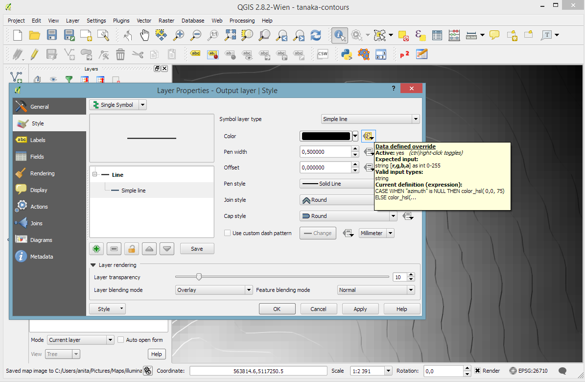
Use the Overlay layer blending mode to blend contours and DEM color:

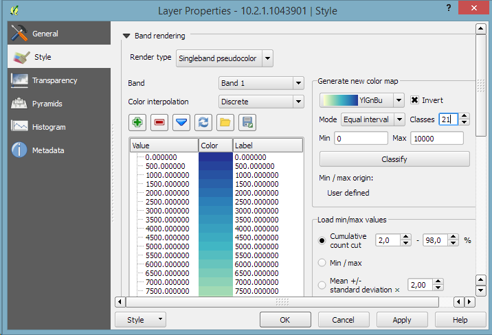
The final step, to get as close to the original design as possible, is to create the effect of discrete elevation classes instead of a smooth color gradient. This can easily be achieved by changing the color interpolation mode of the DEM from Linear to Discrete:

This leaves us with the following gorgeous effect:

As Hannes pointed out, another important aspect of Tanaka’s method is to also alter the contour line width. Lines in the sun or shadow should be wider (1 in this example) than those in orthogonal direction (0.2 in this example):

scale_linear(
abs( abs(
  ( CASE WHEN "azimuth"-45 < 0
    THEN "azimuth"-45+360
    ELSE "azimuth"-45
  END )
-180) -90),
0, 90, 0.2, 1)

Enjoy!