Processing has received a series of updates since the release of QGIS 2.0. (I’m currently running 2.0-20131120) One great addition I want to highlight today is the improved script editor and the help file editor.

Script editor

The improved script editor features a toolbar with commonly used tools such as undo and redo, cut, copy and paste, save and save as …, as well as very useful run algorithm and edit script help buttons. It also shows the script line numbers which makes it easier to work with while debugging code.

The model editor has a similar toolbar now which allows to export the model representation as an image, run the model or edit the model help.

Help editor

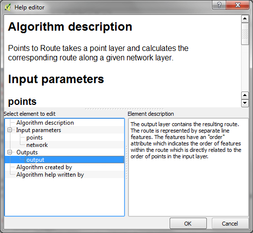
When you press the edit script help button, you get access to the new help editor. It’s easy to use: On the top, it displays the current content of the help file. On the bottom-left, it lists the different sections of the help file which can be filled with information. In the input parameters and outputs section, the help editor automatically lists the all parameters specified in the script code. Finally, in the bottom-right, you can enter the description. The resulting help file is saved in the same location as the original script under the name <scriptname>.py.help.

Update: I’ve revisited this comparison for QGIS 3 in Revisiting point & polygon joins

Joining polygon attributes to points is a pretty common geoprocessing step. There are multiple ways to solve the problem in QGIS, so I thought I’d have a look at how they perform. There is Join attributes by location in the Vector menu and Add polygon attributes to points in the Processing toolbox.

My test data: Two shapefiles with 18,713 points and 17,397 irregular polygons.

(Some system specs: 1.3GHz dualcore with 4GB RAM)

And here are the results:

This point clearly goes to Processing and the SAGA algorithm it provides access to. Join attributes by location offers some nice options for aggregating data but it just can’t cope with the number of features in this test.

To measure execution time (in a very unscientific way), I just ran the tool from the python console using:

import datetime
import processing
print datetime.datetime.now()
processing.runalg("saga:addpolygonattributestopoints","C:/Users/Anita/poi_wien.shp","C:/Users/Anita/REALNUT2009OGD.shp","NUTZUNG_CO",None)
print datetime.datetime.now()

Some notes of caution:
SAGA comes readily installed in OSGeo4W. As far as I know, the stand-alone installer for Windows currently does not include SAGA but it can be installed manually. On Ubuntu, the standard repos only contain SAGA 2.0.8 but 2.1 is required.