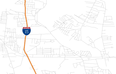
This is a follow-up to my post “Google Maps”-Style Road Maps in QGIS and an answer to @mattwigway’s comment about how to create styles for e.g. US interstates.

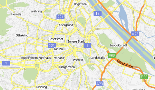
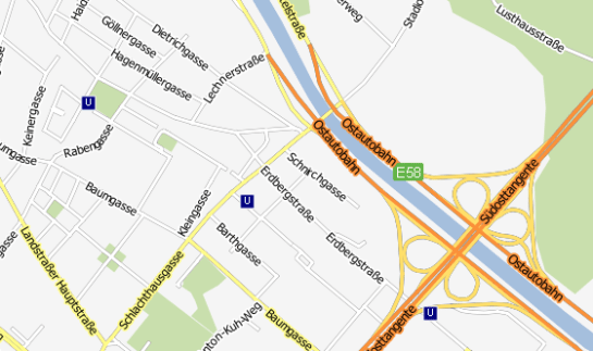
interstate example map

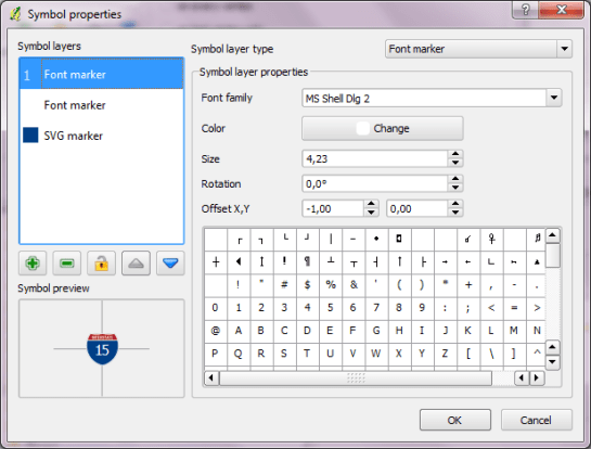
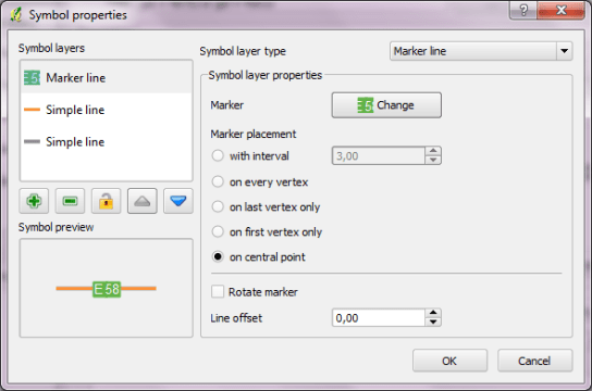
To create a style like this, you can use the “Marker line” feature. The marker can be built using a blank SVG shield and additional text markers to add the road number on top.

creation of the interstate shield marker

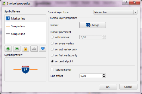
This marker line can be put “on central point” to only show up once along the road.

creation of the interstate style

You can find interstate and other shield style on e.g. Wikimedia Commons. With Inkscape, you can remove the number and thus create a blank marker template.

Tweets to QGIS

By underdark

2011-10-01

GIS, QGIS

9 Comments

The idea behind this post was to create a video of twitter activity using Time Manager. You can watch the results of my first test run here:

And this is how it’s done:

First, you have to collect some tweets with location information. The following command will collect tweets within a certain geographic region from the Twitter Stream API using curl. You need a Twitter user account to use the API. (Curl comes readily available with OSGeo4W install.)

curl -k -d @locations.txt https://stream.twitter.com/1/statuses/filter.json -uuser:password > tweets.json

The contents of locations.txt is the geographic extent you are interested in, e.g. for Austria:

locations=9,45,17,50

After collecting some data, you can load the tweets into QGIS. Executing the following lines in Python Console will add an in-memory point layer to the map. (I am only extracting coordinates and time stamp from the tweets, but you can access more information through the JSON object.)

import simplejson
from PyQt4.QtCore import *
from datetime import *

f=open('C:/temp/tweets.json','r')

# create layer
vl = QgsVectorLayer("Point", "tweets", "memory")
vl.startEditing()
pr = vl.dataProvider()

# add fields
pr.addAttributes( [ QgsField("t", QVariant.String) ] )

# create features
for line in f:
   try:
      j=simplejson.loads(line)
      fet=QgsFeature()
      fet.setGeometry(QgsGeometry.fromPoint(QgsPoint(j['geo']['coordinates'][1],j['geo']['coordinates'][0])))
      fet.setAttributeMap({0:QVariant(str(datetime.strptime(j['created_at'],'%a %b %d %H:%M:%S +0000 %Y')))})
      pr.addFeatures([fet])
   except:
      pass

vl.commitChanges()
vl.updateExtents()

QgsMapLayerRegistry.instance().addMapLayer(vl)

To use the result in Time Manager, you have to export the layer to e.g. Shapefile because it’s not possible to add query strings to in-memory layers.

If you are interested in learning more about PyQGIS, you can find a lot of useful material in the PyQGIS Cookbook.

A Closer Look at Alpha Shapes in pgRouting

By underdark

2011-09-25

PostGIS

2 Comments

Alpha shapes are generalizations of the convex hull [1]. Convex hulls are well known and widely implemented in GIS systems. Alpha shapes are different in that they capture the shape of a point set. You can watch a great demo of how alpha shapes work on François Bélair’s website “Everything You Always Wanted to Know About Alpha Shapes But Were Afraid to Ask” I borrowed the following pictures from that site:

Alpha shapes for different values of alpha. The left one equals the convex hull of the point set.

pgRouting comes with an implementation of alpha shapes. There is an alpha shape function: alphashape(sql text) and a convenience wrapper: points_as_polygon(query character varying). The weird thing is that you don’t get to set an alpha value. The only thing supplied to the function is a set of points. Let’s see what kind of results it produces!

Starting point for this experiment is a 10 km catchment zone around node #2699 in my osm road network. Travel costs to nodes are calculated using driving_distance() function. (You can find more information on using this function in Catchment Areas with pgRouting driving_distance().)

CREATE TABLE home_catchment10km AS
SELECT *
   FROM osm_nodes
   JOIN
   (SELECT * FROM driving_distance('
      SELECT gid AS id,
          source,
          target,
          meters AS cost
      FROM osm_roads',
      2699,
      10000,
      false,
      false)) AS route
   ON
   osm_nodes.id = route.vertex_id

After costs are calculated, we can create some alpha shapes. The following queries create the table and insert an alpha shape for all points with a cost of less than 1500:

CREATE TABLE home_isodist (id serial, max_cost double precision);
SELECT AddGeometryColumn('home_isodist','the_geom',4326,'POLYGON',2);

INSERT INTO home_isodist (max_cost, the_geom) (
SELECT 1500, ST_SetSRID(the_geom,4326)
FROM 
  points_as_polygon(
    'SELECT id, ST_X(the_geom) AS x, ST_Y(the_geom) AS y FROM home_catchment10km where cost < 1500'));

In previous posts, I’ve created catchment areas by first interpolating a cost raster and creating contours from there. Now, let’s see how the two different approaches compare!

The following picture shows resulting catchment areas for 500, 1000, 1500, and 2000 meters around a central node. Colored areas show the form of pgRouting alpha shape results. Black contours show the results of the interpolation method:

Comparison of pgRouting alpha shapes and interpolation method

At first glance, results look similar enough. Alpha shape results look like a generalized version of interpolation results. I guess that it would be possible to get even closer if the alpha value could be set to a smaller value. The function should then produce a finer, more detailed polygon.

For a general overview about which areas of a network are reachable within certain costs, pgRouting alpha shapes function seems a viable alternative to the interpolation method presented in previous posts. However, the alpha value used by pgRouting seems too big to produce detailed catchment areas.

[1] http://biogeometry.duke.edu/software/alphashapes/

“Google Maps”-Style Road Maps in QGIS

By underdark

2011-09-16

Cartography, OSM, QGIS

3 Comments

This is a follow up post on “Guide to Advanced Labeling for OSM Roads”. This post covers how to create a map that looks similar to the classic Google Maps map based on OSM data.

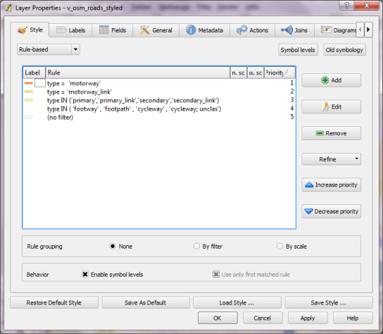
Styling OSM road data is a bit tricky due to the many different possible options in OSM “type” tag. It takes some fiddling around to get results similar to Google. The easiest way to create such a style is using rule-based renderer with “Symbol levels” enabled.

I’ve excluded a number of road types from being rendered and labeled. This is done by NOT specifying a rule that fits those classes. That’s the reason why I don’t have a “no filter” rule. Instead, I’ve specified

type NOT IN ('footway','footpath','steps','cycleway','pedestrian','track','bridleway')

to cover all the roads I don’t want specifically highlighted but displayed using default style. This way I can make sure that footways and similar are neither drawn nor labeled.

Google-style rules for OSM with multiple zoom levels

Now, we can have a look at how to create those road shields Google uses:

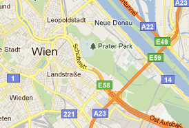
Sample from Google Maps

Currently, it’s not possible to solve this using the labeling engine. And even after labels with “shields” will be implemented, there is still the problem that we want both road names and road numbers labeled – preferably without having to duplicate the layer.

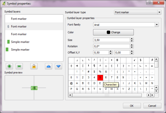
For now, one possible solution for this is to create the shields using the “Marker lines” feature of new symbology. As the name suggests, you can put markers on lines. In this case, the marker will be our road shield. It basically has two parts: the colored shield plus the text. The shield can be created by putting two squares besides each other. (Adjust the offsets to move them besides each other.) Then we can put the text on top, one letter at a time.

Creating the road shield marker

Place the marker on the line once and deactivate “Rotate marker”.

A "road with shield" style

These styles can be assigned to every road you want to decorate with a shield. If you save the style, you just need to change the text next time.

And this is how the result can look like.

Zoomed-out result

Maybe the shields turned out a little too big compared with the original.

Zoomed in, more labels will be displayed and an additional layer with metro stations becomes visible. The metro symbol was created using the same technique described for the road shields.

Zoomed-in result

One disadvantage of creating road shields with this technique – besides the fact that it’s rather tedious – is that there is no collision detection between labels and shields. Nonetheless, it’s a viable solution that allows you to create high-resolution maps that look very similar to Google Maps using free OSM data.

Guide to Advanced Labeling for OSM Roads

By underdark

2011-09-13

Cartography, OSM, PostGIS, QGIS

9 Comments

Advanced labeling in QGIS new labeling engine is mostly about data-defined settings. Almost any property of the label can be controlled.

For this example, we will try to mimic the look of the classic Google map with it’s line and label styles. The data for this post is from the OpenStreetMap project provided as Shapefiles by Cloudmade.

After importing the roads into PostGIS using PostGIS Manager Plugin, we can create a view that will contain the necessary label style information. The trick here is to use CASE statements to distinguish between different label “classes”. Motorway labels will be bigger than the rest and the buffer color will be the same color as used for the corresponding lines.

DROP VIEW IF EXISTS v_osm_roads_styled;

CREATE VIEW v_osm_roads_styled AS
SELECT *, 
CASE WHEN type = 'motorway' THEN 9
     ELSE 8 END
     as font_size,
'black'::TEXT as font_color,
false as font_bold,
false as font_italic,
false as font_underline,
false as font_strikeout,
false as font_family,
1 as buffer_size,
CASE WHEN type = 'motorway' THEN '#fb9139'::TEXT
     WHEN type IN ( 'primary','primary_link','secondary','secondary_link') THEN '#fffb8b'::TEXT
     ELSE 'white'::TEXT END 
     as buffer_color
FROM osm_roads;

In QGIS, we can then load the view and start styling. First, let’s get the line style ready. Using rule-based renderer, it’s easy to create complex styles. In this case, I’ve left it rather simple and don’t distinguish between different zoom levels. That’s a topic for another post :)

Google-style rules for OSM road data

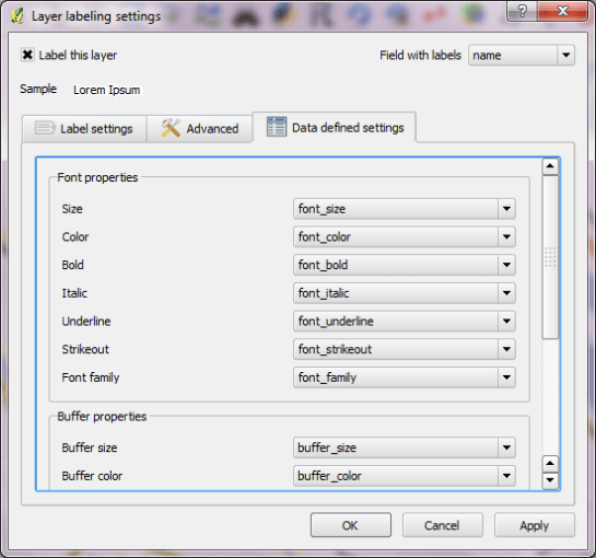
Now for the labels! In “Data defined settings”, we can assign the special attributes created in the database view to the settings.

Completed "Data defined settings"

To achieve an even better look, go to “Advanced” tab and enable “curved” and “on line” placement. “Merge connected lines to avoid duplicate labels” option is very helpful too.

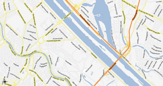
Finally – after adding some water objects (Cloudmade natural.shp) – this is what our result looks like:

Google-style OSM map

This solution can be improved considerably by adding multiple zoom levels with corresponding styles. One obvious difference between the original Google map and this look-alike is the lack of road numbers. Tim’s post on “shield labels” can be a starting point for adding road numbers the way Google does.

QGIS Time Manager Example: Visualizing Storm Data

By underdark

2011-09-06

QGIS, spatio-temporal data, Visualization

Today, I’ve compiled a short video showcasing one of the possible uses of Time Manager plugin: Storm tracking. (Storm data can be downloaded from www.nhc.noaa.gov.)

Point size shows storm class, labels read maximum speed in mph.

If you are using Time Manager for your work, I’d love to hear about it.

Editing Labels in QGIS SVG Output using Inkscape

By underdark

2011-09-01

QGIS

1 Comment

If you are planning to tweak the labels in SVG output from QGIS, you should use the old labeling engine. Labels create with the old engine are written into the SVG file as text objects whereas labels from the new engine end up as paths for some reason.

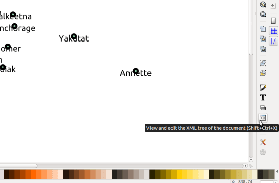
Let’s see how it works using the climate Shapefile from QGIS sample data. I just created an empty map, loaded the points and labeled them before exporting the map to SVG using Print Composer. Now, we can manipulate the SVG file in Inkscape: Select one of the labels and and start the XML Editor (Edit menu – XML Editor or through the toolbar button).

Find the "XML tree" button for full control of the labels

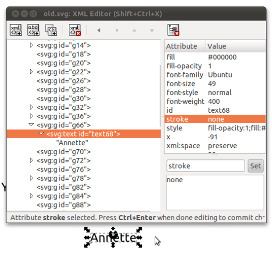
If you selected a label before opening XML Editor, one of the entires in the tree should be highlighted. Expanding the element reveals that it’s a text featuring a series of attributes QGIS exported. From here, you can change both the looks and the text of all labels in your map. Of course, you are not limited to the XML Editor but can change to the GUI – which is certainly recommended for experimenting with all the different settings.

Here you have full control over how the label looks like

Visualizing Global Connections

By underdark

2011-08-20

GIS, PostGIS, QGIS, Visualization

19 Comments

Today, I’ve been experimenting with data from OpenFlights.org. They offer airport, airline and route data for download. The first idea that came to mind was to connect airports on a shared route by lines. This kind of visualization just looks much nicer if the connections are curved instead of simple straight lines.

Luckily, that’s pretty easy to do using PostGIS. After loading airport positions and route data, we can create the connection lines like this (based on [postgis-users] Great circle as a linestring):

UPDATE experimental.airroutes
SET the_geom = 
(SELECT ST_Transform(ST_Segmentize(ST_MakeLine(
       ST_Transform(a.the_geom, 953027),
       ST_Transform(b.the_geom, 953027)
     ), 100000 ), 4326 ) 
 FROM experimental.airports a, experimental.airports b
 WHERE a.id = airroutes.source_id  
   AND b.id = airroutes.dest_id
);

The CRS used in the query is not available in PostGIS by default. You can add it like this (source: spatialreference.org):

INSERT into spatial_ref_sys (srid, auth_name, auth_srid, proj4text, srtext) values ( 953027, 'esri', 53027, '+proj=eqdc +lat_0=0 +lon_0=0 +lat_1=60 +lat_2=60 +x_0=0 +y_0=0 +a=6371000 +b=6371000 +units=m +no_defs ', 'PROJCS["Sphere_Equidistant_Conic",GEOGCS["GCS_Sphere",DATUM["Not_specified_based_on_Authalic_Sphere",SPHEROID["Sphere",6371000,0]],PRIMEM["Greenwich",0],UNIT["Degree",0.017453292519943295]],PROJECTION["Equidistant_Conic"],PARAMETER["False_Easting",0],PARAMETER["False_Northing",0],PARAMETER["Central_Meridian",0],PARAMETER["Standard_Parallel_1",60],PARAMETER["Standard_Parallel_2",60],PARAMETER["Latitude_Of_Origin",0],UNIT["Meter",1],AUTHORITY["EPSG","53027"]]');

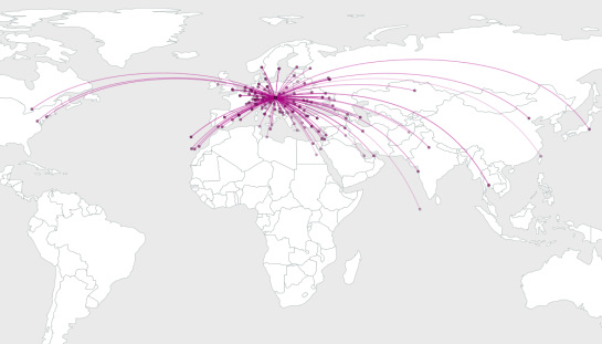
This is an example visualization (done in QGIS) showing only flight routes starting from Vienna International Airport:

Flight routes from Vienna International

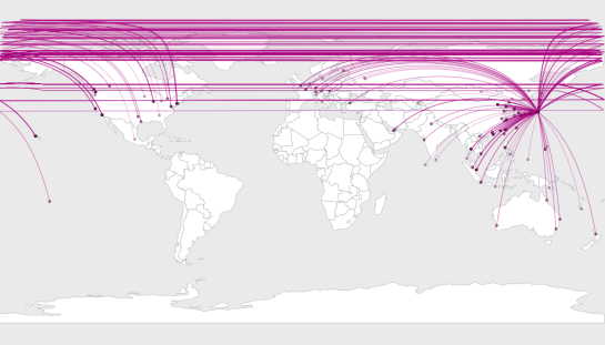
Connections crossing the date line are currently more problematic. Lines would have to be split, otherwise this is what you’ll get:

Date line trouble

How to create a Table with Geometry Column in PostGIS

By underdark

2011-08-15

PostGIS, QGIS

2 Comments

Do you need to create a table with a geometry column in PostGIS from scratch?
Can’t remember the syntax of AddGeometryColumn(varchar catalog_name, varchar schema_name, varchar table_name, varchar column_name, integer srid, varchar type, integer dimension)? I can’t. ;)

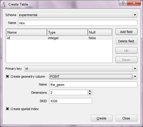
Let’s make our lives easier: QGIS PostGIS Manager offers a convenient GUI for creating tables with geometry columns:

PostGIS Manager Create Table dialog

The dialog works a lot like what you’re probably used to in pgAdmin – with the added nicety of supporting Geometry columns.

In my opinion, this is the fastest way so far to create a spatially enabled table. It provides a much better user experience than telling users (especially new ones) to use AddGeometryColumn(…

Creating a Gradient Fill for Polygons in QGIS

By underdark

2011-08-08

QGIS

2 Comments

QGIS styling options have advanced a lot in the last releases. But there’s always something more we would love to have … Greedy users!

Inkscape and other graphics programs can do it: Gradient fills.

Inspired by a question on gis.stackexchange, I tried to create something as close to a gradient fill as possible.

What I came up with is a symbol consisting out of multiple stacked “simple line” layers. The top-most layer is the dark outer border and every following layer is getting lighter and growing towards the center of the polygon (using a positive offset value). Important options are flat cap styles for all line layers and – of course – enabled symbol levels.

A "gradient" fill in QGIS

As you can see, the gradient looks quite fine inside the polygons. For the edges, it would be necessary to add a mask hiding the unclean rendering. Or maybe there is another solution which I just couldn’t think of?

Nicer map using a mask

This is the symbol source if you want to try it. Paste it into your symbology-ng-style.xml document.

    <symbol outputUnit="MM" alpha="1" type="fill" name="gradient">
      <layer pass="0" class="SimpleFill" locked="0">
        <prop k="color" v="255,255,255,255"/>
        <prop k="color_border" v="0,0,0,255"/>
        <prop k="offset" v="0,0"/>
        <prop k="style" v="solid"/>
        <prop k="style_border" v="solid"/>
        <prop k="width_border" v="1"/>
      </layer>
      <layer pass="0" class="SimpleLine" locked="0">
        <prop k="capstyle" v="flat"/>
        <prop k="color" v="240,240,240,255"/>
        <prop k="customdash" v="5;2"/>
        <prop k="joinstyle" v="bevel"/>
        <prop k="offset" v="6"/>
        <prop k="penstyle" v="solid"/>
        <prop k="use_custom_dash" v="0"/>
        <prop k="width" v="6"/>
      </layer>
      <layer pass="0" class="SimpleLine" locked="0">
        <prop k="capstyle" v="flat"/>
        <prop k="color" v="220,220,220,255"/>
        <prop k="customdash" v="5;2"/>
        <prop k="joinstyle" v="bevel"/>
        <prop k="offset" v="5.5"/>
        <prop k="penstyle" v="solid"/>
        <prop k="use_custom_dash" v="0"/>
        <prop k="width" v="5.5"/>
      </layer>
      <layer pass="0" class="SimpleLine" locked="0">
        <prop k="capstyle" v="flat"/>
        <prop k="color" v="200,200,200,255"/>
        <prop k="customdash" v="5;2"/>
        <prop k="joinstyle" v="bevel"/>
        <prop k="offset" v="5"/>
        <prop k="penstyle" v="solid"/>
        <prop k="use_custom_dash" v="0"/>
        <prop k="width" v="5"/>
      </layer>
      <layer pass="0" class="SimpleLine" locked="0">
        <prop k="capstyle" v="flat"/>
        <prop k="color" v="180,180,180,255"/>
        <prop k="customdash" v="5;2"/>
        <prop k="joinstyle" v="bevel"/>
        <prop k="offset" v="4.5"/>
        <prop k="penstyle" v="solid"/>
        <prop k="use_custom_dash" v="0"/>
        <prop k="width" v="4.5"/>
      </layer>
      <layer pass="0" class="SimpleLine" locked="0">
        <prop k="capstyle" v="flat"/>
        <prop k="color" v="160,160,160,255"/>
        <prop k="customdash" v="5;2"/>
        <prop k="joinstyle" v="bevel"/>
        <prop k="offset" v="4"/>
        <prop k="penstyle" v="solid"/>
        <prop k="use_custom_dash" v="0"/>
        <prop k="width" v="4"/>
      </layer>
      <layer pass="0" class="SimpleLine" locked="0">
        <prop k="capstyle" v="flat"/>
        <prop k="color" v="140,140,140,255"/>
        <prop k="customdash" v="5;2"/>
        <prop k="joinstyle" v="bevel"/>
        <prop k="offset" v="3.5"/>
        <prop k="penstyle" v="solid"/>
        <prop k="use_custom_dash" v="0"/>
        <prop k="width" v="3.5"/>
      </layer>
      <layer pass="0" class="SimpleLine" locked="0">
        <prop k="capstyle" v="flat"/>
        <prop k="color" v="120,120,120,255"/>
        <prop k="customdash" v="5;2"/>
        <prop k="joinstyle" v="bevel"/>
        <prop k="offset" v="3"/>
        <prop k="penstyle" v="solid"/>
        <prop k="use_custom_dash" v="0"/>
        <prop k="width" v="3"/>
      </layer>
      <layer pass="0" class="SimpleLine" locked="0">
        <prop k="capstyle" v="flat"/>
        <prop k="color" v="100,100,100,255"/>
        <prop k="customdash" v="5;2"/>
        <prop k="joinstyle" v="bevel"/>
        <prop k="offset" v="2.5"/>
        <prop k="penstyle" v="solid"/>
        <prop k="use_custom_dash" v="0"/>
        <prop k="width" v="2.5"/>
      </layer>
      <layer pass="0" class="SimpleLine" locked="0">
        <prop k="capstyle" v="flat"/>
        <prop k="color" v="80,80,80,255"/>
        <prop k="customdash" v="5;2"/>
        <prop k="joinstyle" v="bevel"/>
        <prop k="offset" v="2"/>
        <prop k="penstyle" v="solid"/>
        <prop k="use_custom_dash" v="0"/>
        <prop k="width" v="2"/>
      </layer>
      <layer pass="1" class="SimpleLine" locked="0">
        <prop k="capstyle" v="flat"/>
        <prop k="color" v="60,60,60,255"/>
        <prop k="customdash" v="5;2"/>
        <prop k="joinstyle" v="bevel"/>
        <prop k="offset" v="1.5"/>
        <prop k="penstyle" v="solid"/>
        <prop k="use_custom_dash" v="0"/>
        <prop k="width" v="1.5"/>
      </layer>
      <layer pass="2" class="SimpleLine" locked="0">
        <prop k="capstyle" v="flat"/>
        <prop k="color" v="40,40,40,255"/>
        <prop k="customdash" v="5;2"/>
        <prop k="joinstyle" v="bevel"/>
        <prop k="offset" v="1"/>
        <prop k="penstyle" v="solid"/>
        <prop k="use_custom_dash" v="0"/>
        <prop k="width" v="1"/>
      </layer>
      <layer pass="3" class="SimpleLine" locked="0">
        <prop k="capstyle" v="flat"/>
        <prop k="color" v="20,20,20,255"/>
        <prop k="customdash" v="5;2"/>
        <prop k="joinstyle" v="bevel"/>
        <prop k="offset" v="0.5"/>
        <prop k="penstyle" v="solid"/>
        <prop k="use_custom_dash" v="0"/>
        <prop k="width" v="1"/>
      </layer>
      <layer pass="4" class="SimpleLine" locked="0">
        <prop k="capstyle" v="flat"/>
        <prop k="color" v="10,10,10,255"/>
        <prop k="customdash" v="5;2"/>
        <prop k="joinstyle" v="bevel"/>
        <prop k="offset" v="0"/>
        <prop k="penstyle" v="solid"/>
        <prop k="use_custom_dash" v="0"/>
        <prop k="width" v="0.5"/>
      </layer>
    </symbol>