In the past, network analysis capabilities in QGIS were rather limited or not straight-forward to use. This has changed! In QGIS 3.x, we now have a wide range of network analysis tools, both for use case where you want to use your own network data, as well as use cases where you don’t have access to appropriate data or just prefer to use an existing service.
This blog post aims to provide an overview of the options:
- Based on local network data
- Default QGIS Processing network analysis tools
- QNEAT3 plugin
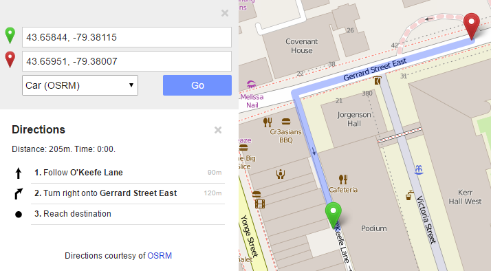
- Based on web services
- Hqgis plugin (HERE)
- ORS Tools plugin (openrouteservice.org)
- TravelTime platform plugin (TravelTime platform)
All five options provide Processing toolbox integration but not at the same level.
If you are a regular reader of this blog, you’re probably also aware of the pgRoutingLayer plugin. However, I’m not including it in this list due to its dependency on PostGIS and its pgRouting extension.
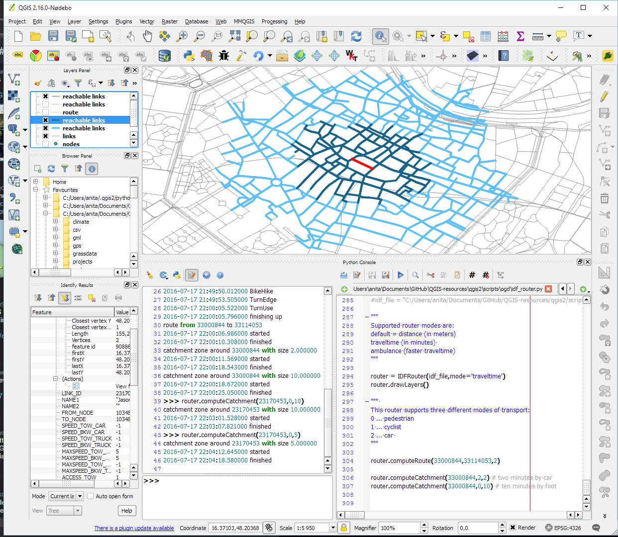
Processing network analysis tools
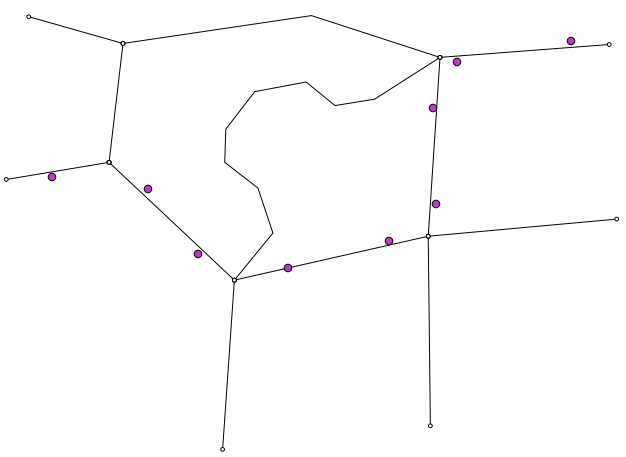
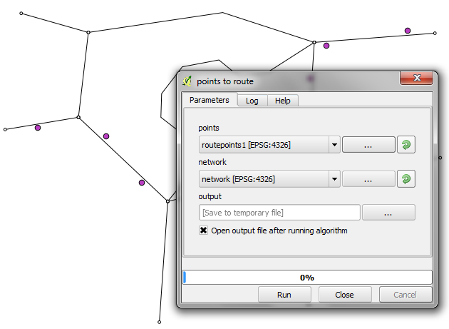
The default Processing network analysis tools are provided out of the box. They provide functionality to compute least cost paths and service areas (distance or time) based on your own network data. Inputs can be individual points or layers of points:
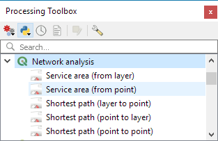
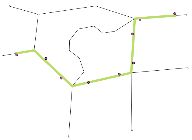
The service area tools return reachable edges and / or nodes rather than a service area polygon:

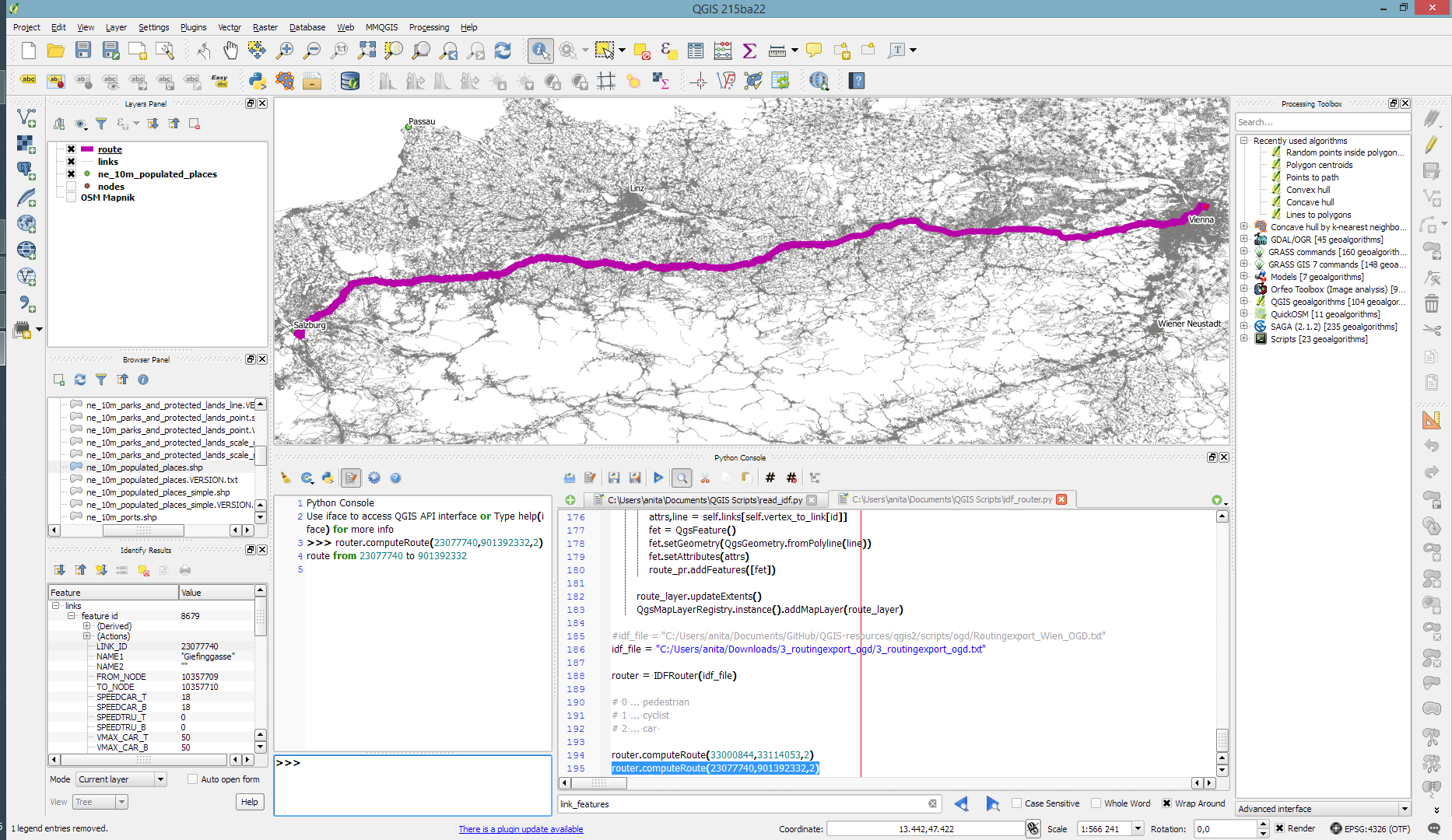
QNEAT3 plugin
The QNEAT3 (short for Qgis Network Analysis Toolbox 3) Plugin aims to provide sophisticated QGIS Processing-Toolbox algorithms in the field of network analysis. QNEAT3 is integrated in the QGIS3 Processing Framework. It offers algorithms that range from simple shortest path solving to more complex tasks like Iso-Area (aka service areas, accessibility polygons) and OD-Matrix (Origin-Destination-Matrix) computation.
QNEAT3 is an alternative for use case where you want to use your own network data.

For more details see the QNEAT3 documentation at: https://root676.github.io/index.html

Hqgis plugin
Access the HERE API from inside QGIS using your own HERE-API key. Currently supports Geocoding, Routing, POI-search and isochrone analysis.
Hqgis currently does not expose all its functionality to the Processing toolbox:
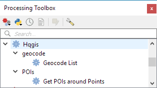
Instead, the full set of functionality is provided through the plugin GUI:

This plugin requires a HERE API key.
ORS Tools plugin
ORS Tools provides access to most of the functions of openrouteservice.org, based on OpenStreetMap. The tool set includes routing, isochrones and matrix calculations, either interactive in the map canvas or from point files within the processing framework. Extensive attributes are set for output files, incl. duration, length and start/end locations.
ORS Tools is based on OSM data. However, using this plugin still requires an openrouteservice.org API key.

TravelTime platform plugin
This plugin adds a toolbar and processing algorithms allowing to query the TravelTime platform API directly from QGIS. The TravelTime platform API allows to obtain polygons based on actual travel time using several transport modes rather, allowing for much more accurate results than simple distance calculations.
The TravelTime platform plugin requires a TravelTime platform API key.


For more details see: https://blog.traveltimeplatform.com/isochrone-qgis-plugin-traveltime