Archive

Author Archives: underdark

We’ve seen a lot of explorative movement data analysis in the Movement data in GIS series so far. Beyond exploration, predictive analysis is another major topic in movement data analysis. One of the most obvious movement prediction use cases is trajectory prediction, i.e. trying to predict where a moving object will be in the future. The two main categories of trajectory prediction methods I see are those that try to predict the actual path that a moving object will take versus those that only try to predict the next destination.

Today, I want to focus on prediction methods that predict the path that a moving object is going to take. There are many different approaches from simple linear prediction to very sophisticated application-dependent methods. Regardless of the prediction method though, there is the question of how to evaluate the prediction results when these methods are applied to real-life data.

As long as we work with nice, densely, and regularly updated movement data, extracting evaluation samples is rather straightforward. To predict future movement, we need some information about past movement. Based on that past movement, we can then try to predict future positions. For example, given a trajectory that is twenty minutes long, we can extract a sample that provides five minutes of past movement, as well as the actually observed position five minutes into the future:

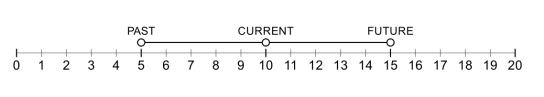
But what if the trajectory is irregularly updated? Do we interpolate the positions at the desired five minute timestamps? Do we try to shift the sample until – by chance – we find a section along the trajectory where the updates match our desired pattern? What if location timestamps include seconds or milliseconds and we therefore cannot find exact matches? Should we introduce a tolerance parameter that would allow us to match locations with approximately the same timestamp?

Depending on the duration of observation gaps in our trajectory, it might not be a good idea to simply interpolate locations since these interpolated locations could systematically bias our evaluation. Therefore, the safest approach may be to shift the sample pattern along the trajectory until a close match (within the specified tolerance) is found. This approach is now implemented in MovingPandas’ TrajectorySampler.

def test_sample_irregular_updates(self):
    df = pd.DataFrame([
        {'geometry':Point(0,0), 't':datetime(2018,1,1,12,0,1)},
        {'geometry':Point(0,3), 't':datetime(2018,1,1,12,3,2)},
        {'geometry':Point(0,6), 't':datetime(2018,1,1,12,6,1)},
        {'geometry':Point(0,9), 't':datetime(2018,1,1,12,9,2)},
        {'geometry':Point(0,10), 't':datetime(2018,1,1,12,10,2)},
        {'geometry':Point(0,14), 't':datetime(2018,1,1,12,14,3)},
        {'geometry':Point(0,19), 't':datetime(2018,1,1,12,19,4)},
        {'geometry':Point(0,20), 't':datetime(2018,1,1,12,20,0)}
        ]).set_index('t')
    geo_df = GeoDataFrame(df, crs={'init': '4326'})
    traj = Trajectory(1,geo_df)
    sampler = TrajectorySampler(traj, timedelta(seconds=5))
    past_timedelta = timedelta(minutes=5)
    future_timedelta = timedelta(minutes=5)
    sample = sampler.get_sample(past_timedelta, future_timedelta)
    result = sample.future_pos.wkt
    expected_result = "POINT (0 19)"
    self.assertEqual(result, expected_result)
    result = sample.past_traj.to_linestring().wkt
    expected_result = "LINESTRING (0 9, 0 10, 0 14)"
    self.assertEqual(result, expected_result)

The repository also includes a demo that illustrates how to split trajectories using a grid and finally extract samples:


In Movement data in GIS #16, I presented a new way to deal with trajectory data using GeoPandas and how to load the trajectory GeoDataframes as a QGIS layer. Following up on this initial experiment, I’ve now implemented a first version of an algorithm that performs a spatial analysis on my GeoPandas trajectories.

The first spatial analysis algorithm I’ve implemented is Clip trajectories by extent. Implementing this algorithm revealed a couple of pitfalls:

  • To achieve correct results, we need to compute spatial intersections between linear trajectory segments and the extent. Therefore, we need to convert our point GeoDataframe to a line GeoDataframe.
  • Based on the spatial intersection, we need to take care of computing the corresponding timestamps of the events when trajectories enter or leave the extent.
  • A trajectory can intersect the extent multiple times. Therefore, we cannot simply use the global minimum and maximum timestamp of intersecting segments.
  • GeoPandas provides spatial intersection functionality but if the trajectory contains consecutive rows without location change, these will result in zero length lines and those cause an empty intersection result.

So far, the clip result only contains the trajectory id plus a suffix indicating the sequence of the intersection segments for a specific trajectory (because one trajectory can intersect the extent multiple times). The following screenshot shows one highlighted trajectory that intersects the extent three times and the resulting clipped trajectories:

This algorithm together with the basic trajectory from points algorithm is now available in a Processing algorithm provider plugin called Processing Trajectory.

Note: This plugin depends on GeoPandas.

Note for Windows users: GeoPandas is not a standard package that is available in OSGeo4W, so you’ll have to install it manually. (For the necessary steps, see this answer on gis.stackexchange.com)

The implemented tests show how to use the Trajectory class independently of QGIS. So far, I’m only testing the spatial properties though:

def test_two_intersections_with_same_polygon(self):
    polygon = Polygon([(5,-5),(7,-5),(7,12),(5,12),(5,-5)])
    data = [{'id':1, 'geometry':Point(0,0), 't':datetime(2018,1,1,12,0,0)},
        {'id':1, 'geometry':Point(6,0), 't':datetime(2018,1,1,12,10,0)},
        {'id':1, 'geometry':Point(10,0), 't':datetime(2018,1,1,12,15,0)},
        {'id':1, 'geometry':Point(10,10), 't':datetime(2018,1,1,12,30,0)},
        {'id':1, 'geometry':Point(0,10), 't':datetime(2018,1,1,13,0,0)}]
    df = pd.DataFrame(data).set_index('t')
    geo_df = GeoDataFrame(df, crs={'init': '31256'})
    traj = Trajectory(1, geo_df)
    intersections = traj.intersection(polygon)
    result = []
    for x in intersections:
        result.append(x.to_linestring())
    expected_result = [LineString([(5,0),(6,0),(7,0)]), LineString([(7,10),(5,10)])]
    self.assertEqual(result, expected_result) 

One issue with implementing the algorithms as QGIS Processing tools in this way is that the tools are independent of one another. That means that each tool has to repeat the expensive step of creating the trajectory objects in memory. I’m not sure this can be solved.

Bugfix release 3.0.2 fixes an issue where “accumulate features” was broken for timestamps with milliseconds.

If you like TimeManager, know your way around setting up Travis for testing QGIS plugins, and want to help improve TimeManager stability, please get in touch!

Many of my previous posts in this series [1][2][3] have relied on PostGIS for trajectory data handling. While I love PostGIS, it feels like overkill to require a database to analyze smaller movement datasets. Wouldn’t it be great to have a pure Python solution?

If we look into moving object data literature, beyond the “trajectories are points with timestamps” perspective, which is common in GIS, we also encounter the “trajectories are time series with coordinates” perspective. I don’t know about you, but if I hear “time series” and Python, I think Pandas! In the Python Data Science Handbook, Jake VanderPlas writes:

Pandas was developed in the context of financial modeling, so as you might expect, it contains a fairly extensive set of tools for working with dates, times, and time-indexed data.

Of course, time series are one thing, but spatial data handling is another. Lucky for us, this is where GeoPandas comes in. GeoPandas has been around for a while and version 0.4 has been released in June 2018. So far, I haven’t found examples that use GeoPandas to manage movement data, so I’ve set out to give it a shot. My trajectory class uses a GeoDataFrame df for data storage. For visualization purposes, it can be converted to a LineString:

import pandas as pd 
from geopandas import GeoDataFrame
from shapely.geometry import Point, LineString

class Trajectory():
    def __init__(self, id, df, id_col):
        self.id = id
        self.df = df    
        self.id_col = id_col
        
    def __str__(self):
        return "Trajectory {1} ({2} to {3}) | Size: {0}".format(
            self.df.geometry.count(), self.id, self.get_start_time(), 
            self.get_end_time())
        
    def get_start_time(self):
        return self.df.index.min()
        
    def get_end_time(self):
        return self.df.index.max()
        
    def to_linestring(self):
        return self.make_line(self.df)
        
    def make_line(self, df):
        if df.size > 1:
            return df.groupby(self.id_col)['geometry'].apply(
                lambda x: LineString(x.tolist())).values[0]
        else:
            raise RuntimeError('Dataframe needs at least two points to make line!')

    def get_position_at(self, t):
        try:
            return self.df.loc[t]['geometry'][0]
        except:
            return self.df.iloc[self.df.index.drop_duplicates().get_loc(
                t, method='nearest')]['geometry']

Of course, this class can be used in stand-alone Python scripts, but it can also be used in QGIS. The following script takes data from a QGIS point layer, creates a GeoDataFrame, and finally generates trajectories. These trajectories can then be added to the map as a line layer.

All we need to do to ensure that our data is ordered by time is to set the GeoDataFrame’s index to the time field. From then on, Pandas takes care of the time series aspects and we can access the index as shown in the Trajectory.get_position_at() function above.

# Get data from a point layer
l = iface.activeLayer()
time_field_name = 't'
trajectory_id_field = 'trajectory_id' 
names = [field.name() for field in l.fields()]
data = []
for feature in l.getFeatures():
    my_dict = {}
    for i, a in enumerate(feature.attributes()):
        my_dict[names[i]] = a
    x = feature.geometry().asPoint().x()
    y = feature.geometry().asPoint().y()
    my_dict['geometry']=Point((x,y))
    data.append(my_dict)

# Create a GeoDataFrame
df = pd.DataFrame(data).set_index(time_field_name)
crs = {'init': l.crs().geographicCrsAuthId()} 
geo_df = GeoDataFrame(df, crs=crs)
print(geo_df)

# Test if spatial functions work
print(geo_df.dissolve([True]*len(geo_df)).centroid)

# Create a QGIS layer for trajectory lines
vl = QgsVectorLayer("LineString", "trajectories", "memory")
vl.setCrs(l.crs()) # doesn't stop popup :(
pr = vl.dataProvider()
pr.addAttributes([QgsField("id", QVariant.String)])
vl.updateFields() 

df_by_id = dict(tuple(geo_df.groupby(trajectory_id_field)))
trajectories = {}
for key, value in df_by_id.items():
    traj = Trajectory(key, value, trajectory_id_field)
    trajectories[key] = traj
    line = QgsGeometry.fromWkt(traj.to_linestring().wkt)
    f = QgsFeature()
    f.setGeometry(line)
    f.setAttributes([key])
    pr.addFeature(f) 
print(trajectories[1])

vl.updateExtents() 
QgsProject.instance().addMapLayer(vl)

The following screenshot shows this script applied to a sample of the Geolife datasets containing 100 trajectories with a total of 236,776 points. On my notebook, the runtime is approx. 20 seconds.

So far, GeoPandas has proven to be a convenient way to handle time series with coordinates. Trying to implement some trajectory analysis tools will show if it is indeed a promising data structure for trajectories.

If you follow me on Twitter, you have probably already heard that the ebook of “QGIS Map Design 2nd Edition” has now been published and we are expecting the print version to be up for sale later this month. Gretchen Peterson and I – together with our editor Gary Sherman (yes, that Gary Sherman!) – have been working hard to provide you with tons of new and improved map design workflows and many many completely new maps. By Gretchen’s count, this edition contains 23 new maps, so it’s very hard to pick a favorite!

Like the 1st edition, we provide increasingly advanced recipes in three chapters, each focusing on either layer styling, labeling, or creating print layouts. If I had to pick a favorite, I’d have to go with “Mastering Rotated Maps”, one of the advanced recipes in the print layouts chapter. It looks deceptively simple but it combines a variety of great QGIS features and clever ideas to design a map that provides information on multiple levels of detail. Besides the name inspiring rotated map items, this design combines

  • map overviews
  • map themes
  • graduated lines and polygons
  • a rotated north arrow
  • fancy leader lines

all in one:

“QGIS Map Design 2nd Edition” provides how-to instructions, as well as data and project files for each recipe. So you can jump right into it and work with the provided materials or apply the techniques to your own data.

The ebook is available at LocatePress.

Need to geocode some addresses? Here’s a five-lines-of-code solution based on “An A-Z of useful Python tricks” by Peter Gleeson:

from geopy import GoogleV3
place = "Krems an der Donau"
location = GoogleV3().geocode(place)
print(location.address)
print("POINT({},{})".format(location.latitude,location.longitude))

For more info, check out geopy:

geopy is a Python 2 and 3 client for several popular geocoding web services.
geopy includes geocoder classes for the OpenStreetMap Nominatim, ESRI ArcGIS, Google Geocoding API (V3), Baidu Maps, Bing Maps API, Yandex, IGN France, GeoNames, Pelias, geocode.earth, OpenMapQuest, PickPoint, What3Words, OpenCage, SmartyStreets, GeocodeFarm, and Here geocoder services.

Do you sometimes start writing an SQL query and around at line 50 you get the feeling that it might be getting out of hand? If so, it might be useful to start breaking it down into smaller chunks and wrap those up into custom functions. Never done that? Don’t despair! There’s an excellent PL/pgSQL tutorial on postgresqltutorial.com to get you started.

To get an idea of the basic structure of a PL/pgSQL function and to proof that PostGIS datatypes work just fine in this context, here’s a basic function that takes a trajectory geometry and outputs its duration, i.e. the difference between its last and first timestamp:

CREATE OR REPLACE FUNCTION AG_Duration(traj geometry) 
RETURNS numeric LANGUAGE 'plpgsql'
AS $BODY$ 
BEGIN
RETURN ST_M(ST_EndPoint(traj))-ST_M(ST_StartPoint(traj));
END; $BODY$;

My end goal for this exercise was to implement a function that takes a trajectory and outputs the stops along this trajectory. Commonly, a stop is defined as a long stay within an area with a small radius. This leads us to the following definition:

CREATE OR REPLACE FUNCTION AG_DetectStops(
   traj geometry, 
   max_size numeric, 
   min_duration numeric)
RETURNS TABLE(sequence integer, geom geometry) 
-- implementation follows here!

Note how this function uses RETURNS TABLE to enable it to return all the stops that it finds. To add a line to the output table, we need to assign values to the sequence and geom variables and then use RETURN NEXT.

Another reason to use PL/pgSQL is that it enables us to write loops. And loops I wanted for my stop detection function! Specifically, I wanted to go through all the points in the trajectory:

FOR pt IN SELECT (ST_DumpPoints(traj)).geom LOOP
-- here comes the magic!
END LOOP;

Eventually the function should go through the trajectory and identify all segments that stay within an area with max_size diameter for at least min_duration time. To test for the area size, we can use:

IF ST_MaxDistance(segment,pt) <= max_size THEN is_stop := true; 

Putting everything together, my current implementation looks like this:

CREATE OR REPLACE FUNCTION AG_DetectStops(traj geometry, max_size numeric, min_duration numeric)
    RETURNS TABLE(sequence integer, geom geometry) LANGUAGE 'plpgsql'
AS $BODY$
DECLARE 
    pt geometry;
    segment geometry;
    is_stop boolean;
    previously_stopped boolean;
    stop_sequence integer;
    p1 geometry;
BEGIN
segment := NULL;
sequence := 0;
is_stop := false;
previously_stopped := false;
p1 := NULL;
FOR pt IN SELECT (ST_DumpPoints(traj)).geom 
LOOP
   IF segment IS NULL AND p1 IS NULL THEN 
      p1 := pt; 
   ELSIF segment IS NULL THEN 
      segment := ST_MakeLine(p1,pt); 
      p1 := NULL;
      IF ST_Length((segment)) <= max_size THEN is_stop := true; END IF;
   ELSE 
      segment := ST_AddPoint(segment,pt); 
      -- if we're in a stop, we want to grow the segment, otherwise we remove points to the specified min_duration
      IF NOT is_stop THEN
         WHILE ST_NPoints(segment) > 2 AND AG_Duration(ST_RemovePoint(segment,0)) >= min_duration LOOP
            segment := ST_RemovePoint(segment,0); 
         END LOOP;
      END IF;
      -- a stop is identified if the segment stays within a circle of diameter = max_size
      IF ST_Length((segment)) <= max_size THEN is_stop := true;  -- not necessary but faster
      ELSIF ST_Distance((ST_StartPoint(segment)),(pt)) > max_size THEN is_stop := false;
      ELSIF ST_MaxDistance(segment,pt) <= max_size THEN is_stop := true;											
      ELSE is_stop := false; 
      END IF;
      -- if we found the end of a stop, we need to check if it lasted long enough
      IF NOT is_stop AND previously_stopped THEN 
         IF ST_M(ST_PointN(segment,ST_NPoints(segment)-1))-ST_M(ST_StartPoint(segment)) >= min_duration THEN
            geom := ST_RemovePoint(segment,ST_NPoints(segment)-1); 
            RETURN NEXT;
            sequence := sequence + 1;
            segment := NULL;
            p1 := pt;
	     END IF;
      END IF;
   END IF;
   previously_stopped := is_stop;
END LOOP;
IF previously_stopped AND AG_Duration(segment) >= min_duration THEN 
   geom := segment; 
   RETURN NEXT; 
END IF;
END; 
$BODY$;	

While this function is not really short, it’s so much more readable than my previous attempts of doing this in pure SQL. Some of the lines for determining is_stop are not strictly necessary but they do speed up processing.

Performance still isn’t quite where I’d like it to be. I suspect that all the adding and removing points from linestring geometries is not ideal. In general, it’s quicker to find shorter stops in smaller areas than longer stop in bigger areas.

Let’s test! 

Looking for a testing framework for PL/pgSQL, I found plpgunit on Github. While I did not end up using it, I did use its examples for inspiration to write a couple of tests, e.g.

CREATE OR REPLACE FUNCTION test.stop_at_beginning() RETURNS void LANGUAGE 'plpgsql'
AS $BODY$
DECLARE t0 integer; n0 integer;
BEGIN
WITH temp AS ( SELECT AG_DetectStops(
   ST_GeometryFromText('LinestringM(0 0 0, 0 0 1, 0.1 0.1 2, 2 2 3)'),
   1,1) stop 
)
SELECT ST_M(ST_StartPoint((stop).geom)), 
       ST_NPoints((stop).geom) FROM temp INTO t0, n0;	
IF t0 = 0 AND n0 = 3
   THEN RAISE INFO 'PASSED - Stop at the beginning of the trajectory';
   ELSE RAISE INFO 'FAILED - Stop at the beginning of the trajectory';
END IF;
END; $BODY$;

Basically, each test is yet another PL/pgSQL function that doesn’t return anything (i.e. returns void) but outputs messages about the status of the test. Here I made heavy use of the PERFORM statement which executes the provided function but discards the results:


Update: The source code for this function is now available on https://github.com/anitagraser/postgis-spatiotemporal

Last week, I traveled to Salzburg to attend the 30th AGIT conference and co-located English-speaking GI_Forum. Like in previous year, there were a lot of mobility and transportation research related presentations. Here are my personal highlights:

This year’s keynotes touched on a wide range of issues, from Sandeep Singhal (Google Cloud Storage) who – when I asked about the big table queries he showed – stated that they are not using a spatial index but are rather brute-forcing their way through massive data sets, to Laxmi Ramasubramanian @nycplanner (Hunter College City University of New York) who cautioned against tech arrogance and tendency to ignore expertise from other fields such as urban planning:

https://twitter.com/underdarkGIS/status/1014412390249697280

One issue that Laxmi particularly highlighted was the fact that many local communities are fighting excessive traffic caused by apps like Waze that suggest shortcuts through residential neighborhoods. Just because we can do something with (mobility) data, doesn’t necessarily mean that we should!

https://twitter.com/underdarkGIS/status/1014898552538005505

Not limited to mobility but very focused on open source, Jochen Albrecht (Hunter College City University of New York) invited the audience to join his quest for a spatial decision support system based on FOSS only at bit.ly/FiltersAndWeights and https://github.com/geojochen/fosssdss

https://twitter.com/underdarkGIS/status/1014890452775067650

The session Spatial Perspectives on Healthy Mobility featured multiple interesting contributions, particularly by Michelle P. Fillekes who presented a framework of mobility indicators to assess daily mobility of study participants. It considers both spatial and temporal aspects of movement, as well as the movement context:

Figure from Michelle Pasquale Fillekes, Eleftheria Giannouli, Wiebren Zijlstra, Robert Weibel. Towards a Framework for Assessing Daily Mobility using GPS Data. DOI: 10.1553/giscience2018_01_s177 (under cc-by-nd)

It was also good to see that topics we’ve been working on in the past (popularity routing in this case) continue to be relevant and have been picked up in the German-speaking part of the conference:

Of course, I also presented some new work of my own, specifically my research into PostGIS trajectory datatypes which I’ve partially covered in a previous post on this blog and which is now published in Graser, A. (2018) Evaluating Spatio-temporal Data Models for Trajectories in PostGIS Databases. GI_Forum ‒ Journal of Geographic Information Science, 1-2018, 16-33. DOI: 10.1553/giscience2018_01_s16.

My introduction to GeoMesa talk failed to turn up any fellow Austrian GeoMesa users. So I’ll keep on looking and spreading the word. The most common question – and certainly no easy one at that – is how to determine the point where it becomes worth it to advance from regular databases to big data systems. It’s not just about the size of the data but also about how it is intended to be used. And of course, if you are one of those db admin whizzes who manages a distributed PostGIS setup in their sleep, you might be able to push the boundaries pretty far. On the other hand, if you already have some experience with the Hadoop ecosystem, getting started with tools like GeoMesa shouldn’t be too huge a step either. But that’s a topic for another day!

Since AGIT&GI_Forum are quite a big event with over 1,000 participants, it was not limited to movement data topics. You can find the first installment of English papers in GI_Forum 2018, Volume 1. As I understand it, there will be a second volume with more papers later this year.


This post is part of a series. Read more about movement data in GIS.

If you’re are following me on Twitter, you’ve certainly already read that I’m working on PyQGIS 101 a tutorial to help GIS users to get started with Python programming for QGIS.

https://twitter.com/underdarkGIS/status/1002287546464919552

I’ve often been asked to recommend Python tutorials for beginners and I’ve been surprised how difficult it can be to find an engaging tutorial for Python 3 that does not assume that the reader already knows all kinds of programming concepts.

It’s been a while since I started programming, but I do teach QGIS and Python programming for QGIS to university students and therefore have some ideas of which concepts are challenging. Nonetheless, it’s well possible that I overlook something that is not self explanatory. If you’re using PyQGIS 101 and find that some points could use further explanations, please leave a comment on the corresponding page.

PyQGIS 101 is a work in progress. I’d appreciate any feedback, particularly from beginners!

Working with movement data analysis, I’ve banged my head against performance issues every once in a while. For example, PostgreSQL – and therefore PostGIS – run queries in a single thread of execution. This is now changing, with more and more functionality being parallelized. PostgreSQL version 9.6 (released on 2016-09-29) included important steps towards parallelization, including parallel execution of sequential scans, joins and aggregates. Still, there is no parallel processing in PostGIS so far (but it is under development as described by Paul Ramsey in his posts “Parallel PostGIS II” and “PostGIS Scaling” from late 2017).

At the FOSS4G2016 in Bonn, I had the pleasure to chat with Shoaib Burq who ran the “An intro to Apache PySpark for Big Data GeoAnalysis” workshop. Back home, I downloaded the workshop material and gave it a try but since I wanted a scalable system for storing, analyzing, and visualizing spatial data, it didn’t really seem to fit the bill.

Around one year ago, my search grew more serious since we needed a solution that would support our research group’s new projects where we expected to work with billions of location records (timestamped points and associated attributes). I was happy to find that the fine folks at LocationTech have some very promising open source projects focusing on big spatial data, most notably GeoMesa and GeoWave. Both tools take care of storing and querying big spatio-temporal datasets and integrate into GeoServer for publication and visualization. (A good – if already slightly outdated – comparison of the two has been published by Azavea.)

My understanding at the time was that GeoMesa had a stronger vector data focus while GeoWave was more focused on raster data. This lead me to try out GeoMesa. I published my first steps in “Getting started with GeoMesa using Geodocker” but things only really started to take off once I joined the developer chats and was pointed towards CCRI’s cloud-local “a collection of bash scripts to set up a single-node cloud on your desktop, laptop, or NUC”. This enabled me to skip most of the setup pains and go straight to testing GeoMesa’s functionality.

The learning curve is rather significant: numerous big data stack components (including HDFS, Accumulo, and GeoMesa), a most likely new language (Scala), as well as the Spark computing system require some getting used to. One thing that softened the blow is the fact that writing queries in SparkSQL + GeoMesa is pretty close to writing PostGIS queries. It’s also rather impressive to browse hundreds of millions of points by connecting QGIS TimeManager to a GeoServer WMS-T with GeoMesa backend.

Spatial big data stack with GeoMesa

One of the first big datasets I’ve tested are taxi floating car data (FCD). At one million records per day, the three years in the following example amount to a total of around one billion timestamped points. A query for travel times between arbitrary start and destination locations took a couple of seconds:

Travel time statistics with GeoMesa (left) compared to Google Maps predictions (right)

Besides travel time predictions, I’m also looking into the potential for predicting future movement. After all, it seems not unreasonable to assume that an object would move in a similar fashion as other similar objects did in the past.

Early results of a proof of concept for GeoMesa based movement prediction

Big spatial data – both vector and raster – are an exciting challenge bringing new tools and approaches to our ever expanding spatial toolset. Development of components in open source big data stacks is rapid – not unlike the development speed of QGIS. This can make it challenging to keep up but it also holds promises for continuous improvements and quick turn-around times.

If you are using GeoMesa to work with spatio-temporal data, I’d love to hear about your experiences.