A very common approach for mapping point density is to use heat maps. If you are aiming for a different style, give hexagonal grids a try. The workflow is very simple in QGIS:

Load the point layer
Create a hexagonal grid using MMQGIS – Create Grid Layer
Count points per polygon (Vector menu)

I’ve applied this method to an OGD dataset of the Viennese tree cadastre containing 119,744 tree positions:

Default style: One dot per tree

Rendering tree counts per hexagonal grid cell reveals some of Vienna’s greenest spots, such as the Prater or Türkenschanzpark.

Tree density in a hexagonal grid

There’s also a printable version.

Some notes on the necessary steps:

MMQGIS – Create Grid Layer performs great. Creating the 18,400 hexagons in this map was very fast. Note though, that this tool doesn’t seem to write correct projection information to the resulting Shapefile. Therefore it is necessary to set the projection manually after loading the file.

As a result, it is very likely that the Points in Polygon tool will warn you that the point and polygon layer are not in the same projection. I ignored the warning and everything went fine. This step was reasonably fast considering the number of points (119,744) and polygons (18,400).

Light Styles for OSM Layers in QGIS

By underdark

2012-02-25

OSM, QGIS

47 Comments

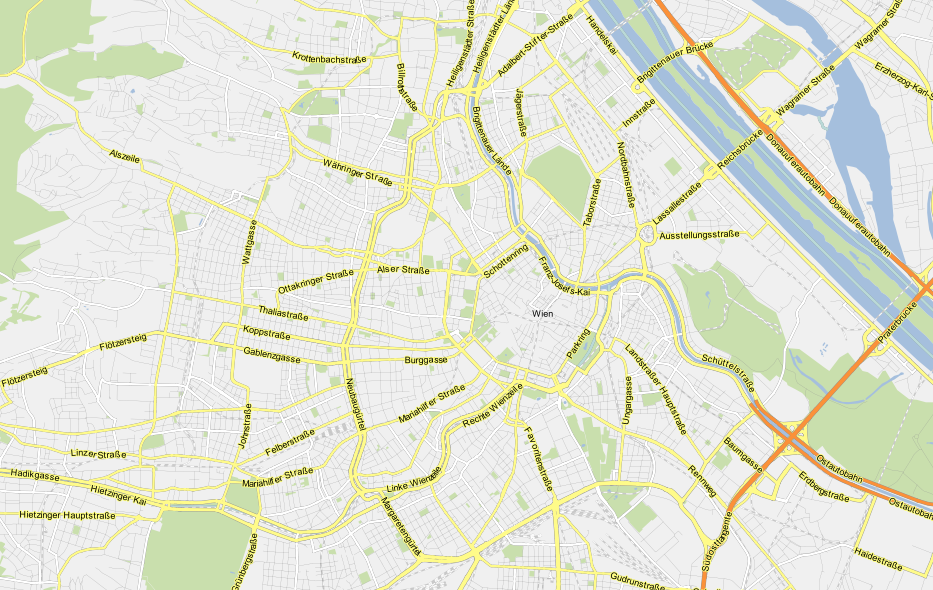
The default look of OSM plugin layers is not well-suited for background map usage. It’s too colorful and any overlay just gets lost:

Default look of OSM plugin layers

A good background map has enough detail to allow the reader to orient himself but at the same time must not overwhelm the overlays. For data to be overlaid onto OSM plugin layers, a more neutral style is needed. And this is my first attempt at such a style, containing rules for the polygon and line layers (no point style yet):

Light OSM style applied to polygon and line layer

As before, these styles can be downloaded from my “QGIS-resources” Github repository. They are called osm_light_line.qml and osm_light_polygon.qml and require QGIS trunk. They do not work in QGIS 1.7.x because they contain some new features that are only available in the developer version (aka trunk).

New Download: Osm2po Light Style

By underdark

2012-02-18

QGIS

24 Comments

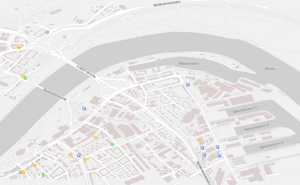
Inspired by the “OSM Bright Minimal” style for Tilemill, I’ve created a similar background map style for osm2po layers in QGIS trunk (uses features unavailable in 1.7.3): osm2po_light_style.qml. Together with a grey background (RGB:232,232,232) and an OSM natural layer (RGB:208,208,208 for water), the style looks like this:

example map using osm2po_light_style.qml

It’s plain and bright, so any overlay will stand out nicely. Hope you find it useful.

Batch Application of QGIS Layer Styles

By underdark

2012-02-17

QGIS

Ever had to apply the same style to multiple map layers? It’s a tedious task … if you don’t have MultiQML plugin by Gislab.

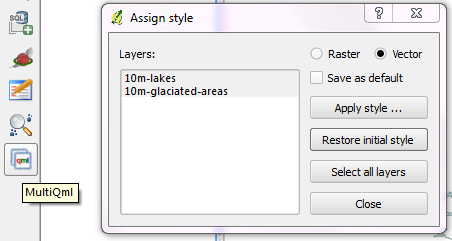
With MultiQML, you can apply a style to multiple raster or vector layers: First, select the layers you want to style (use shift/ctrl to select multiple layers), press “Apply style …” button and select the appropriate QML. That’s it!

MultiQML dialog

The tool even has an “undo” functionality called “Restore initial style”, which will certainly prove useful.

If you want to see MultiQML in action, Gislab provides a video tutorial on their plugin page.

New Download: Osm2po Style

By underdark

2012-02-15

OSM, QGIS

7 Comments

Please read the new instructions for QGIS 2.

I’ve added a new style for osm2po layers to the QGIS Resources Github repo. It contains the following rules:

the rules

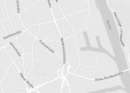
and looks like this:

the map

Enjoy!

A Guide to Beautiful Reliefs in QGIS

By underdark

2012-01-19

GIS, QGIS

10 Comments

This week Sourcepole released a new addition to the Raster Terrain Analysis plugin: a sophisticated Relief tool. (More info in their announcement) This plugin is shipped with QGIS (developer version, not in 1.7.3 release) by default but you might have to activate it in Plugin Manager:

The plugin dialog is quite self-explanatory. You can chose the elevation file, output path and any of the numerous raster formats. The z factor is a bit more mysterious. We will have a look at that in a second. The rest of the dialog is the relief color editor. Pressing Create automatically will give you a color gradient to start with.

Relief tool dialog

But what’s the z factor good for?

I’ve tried a few different settings using free NASA SRTM data and it seems that higher values lead to a smoother relief (Please ignore the water areas):

z factor = 100

z factor = 1000

z factor = 10000

z factor = 50000

z factor = 100000

Update:

As Marco noted in the comments: The z factor is used if the x/y units are different from the z unit.

If everything is in meters, use z factor 1.0 (default).
If x/y is in degree and z in meters, use z factor 111120.
If x/y degree and z is feet, use z factor 370400.

In the example above SRTM rasters are in WGS84 with heights in meters. That’s why the result using a z factor of 100000 looks so good.

In my opinion the results look great even with the coarse SRTM dataset I used. Looking forward to all the great QGIS maps we will see in the future.

Easier Conditional Labels in QGIS

By underdark

2012-01-09

QGIS

4 Comments

With Martin’s latest addition of conditional statements it’s now even easier to get conditional labels in QGIS. Following up on the example used in my previous post, we can simplify

substr(osm_name, 0, (clazz = 11 or clazz = 13 or clazz = 15 or clazz = 21)*-1)

to

CASE WHEN (clazz = 11 or clazz = 13 or clazz = 15 or clazz = 21) THEN osm_name END

which is much easier to read and remember.

To avoid roads from being labeled with only their road numbers, I added an additional check that the “osm_name” is longer than six characters. Thanks to Nathan’s syntax highlighting this new and powerful expression based labeling is also comfortable to use.

Conditional labels for an osm2po layer

Conditional Labels in QGIS

By underdark

2011-12-30

QGIS

4 Comments

The latest QGIS development build (1.9.90) has a new feature “expression based labeling” which can be used to create conditional labels. One typical use case would be if you want to label only certain (high-level) road classes in your road layer. By default, QGIS labels the features rather randomly:

default labeling

How can we label only the more important roads? Here is an example using OSM data imported into PostGIS using osm2po:

If you have loaded OSM using osm2po, your OSM table will contain a “clazz” attribute. (Check osm2po.config for the exact mapping.) To label only motorways, trunks, primary and secondary roads and nothing else, I wrote this labeling expression:

substr(osm_name, 0, (clazz = 11 or clazz = 13 or clazz = 15 or clazz = 21)*-1)

If clazz equals 11, 13, 15 or 21, the expression returns the value of osm_name. Otherwise it returns an empty string. (All checks will return false or 0 which causes the function to evaluate to substr(osm_name,0,0).) Kudos to Giuseppe Sucameli who explained this on the mailing list.

expression based "conditional" labels

Mapping QGIS Users

By underdark

2011-12-27

QGIS, Visualization

5 Comments

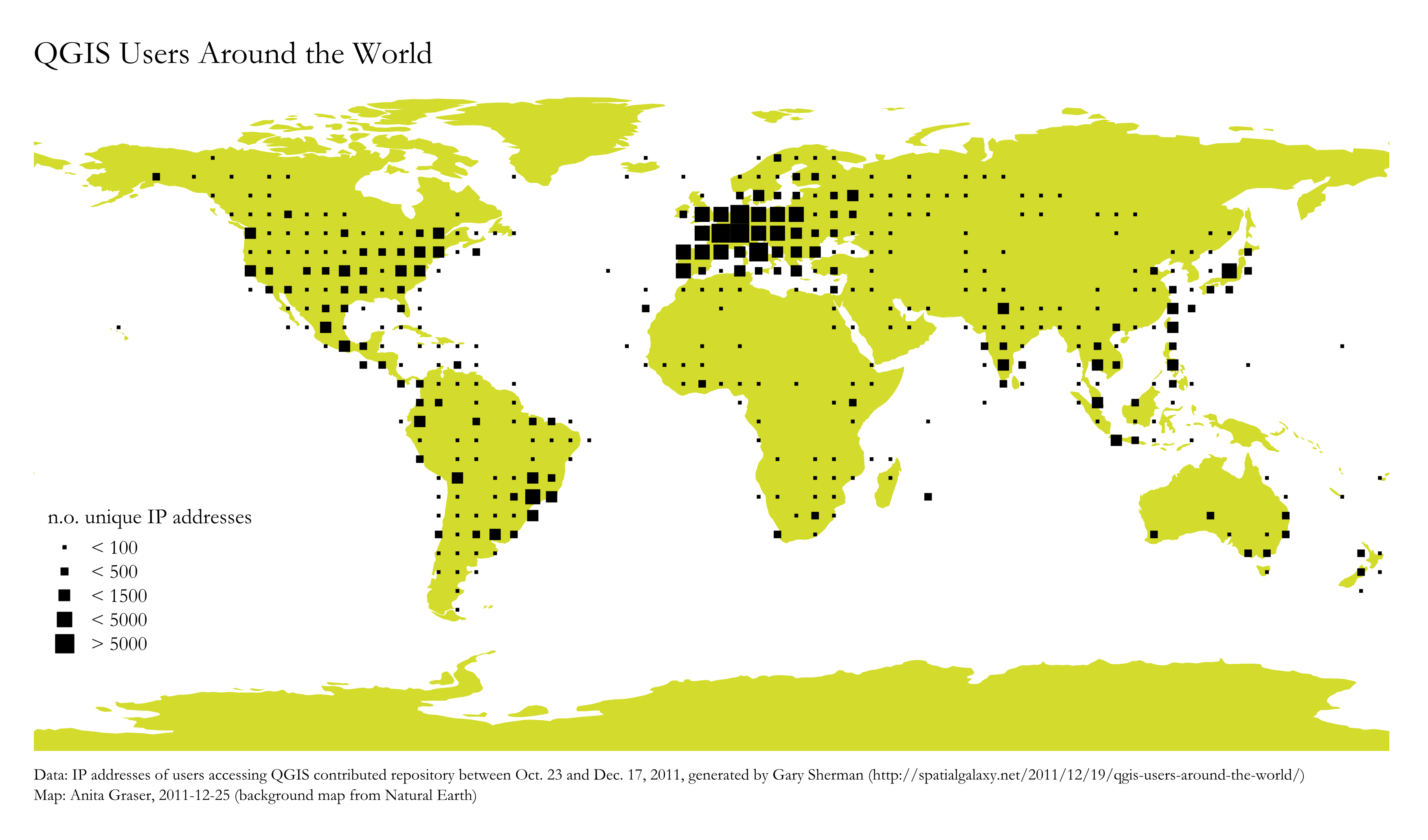
For “QGIS Users Around the World” Gary Sherman collected and geocoded a few weeks of accesses to the plugin repositories. This map is my first attempt at mapping the data for use in QGIS publications:

Considering the coarse resolution of geocoded IP addresses, I’ve decided to count the number of unique IP addresses within each area (5×5 degrees). We can make out a lot of activity in Europe, Japan, Brazil and the US. The high number of accesses from the US mid west are due to IPs being mapped to country-level only.

I would love to hear your feedback on this one!

TimeManager is now on Github

By underdark

2011-12-27

QGIS

TimeManager is now available on Github (right beside pgRoutingLayer).

If you want to try it, you can install version 0.4 from the new QGIS Plugin Repository. I’ve also uploaded some test data such as the twitter file used for the animation I presented recently.