Today, I’m super excited to share with you the announcement that our open source textbook “Geocomputation with Python” has finally arrived in print and is now available for purchase from Routledge.com, Amazon.com, Amazon.co.uk, and other booksellers.

“Geocomputation with Python” (or geocompy for short) covers the entire range of standard GIS operations for both vector and raster data models. Each section and chapter builds on the previous. If you’re just starting out with Python to work with geographic data, we hope that the book will be an excellent place to start.

Of course, you can still find the online version of the book at py.geocompx.org.

The book is open-source and you can find the code on GitHub. This ensures that the content is reproducible, transparent, and accessible. It also lets you interact with the project by opening issues and submitting pull requests.

GeoParquet in QGIS – smaller & faster files for the win!

By underdark

2024-11-23

Big Data, GIS, Movement data in GIS, QGIS

5 Comments

tldr; Tired of working with large CSV files? Give GeoParquet a try!

“Parquet is a powerful column-oriented data format, built from the ground up to as a modern alternative to CSV files.” https://geoparquet.org/

(Geo)Parquet is both smaller and faster than CSV. Additionally, (Geo)Parquet columns are typed. Text, numeric values, dates, geometries retain their data types. GeoParquet also stores CRS information and support in GIS solutions is growing.

I’ll be giving a quick overview using AIS data in GeoPandas 1.0.1 (with pyarrow) and QGIS 3.38 (with GDAL 3.9.2).

File size

The example AIS dataset for this demo contains ~10 million rows with 22 columns. I’ve converted the original zipped CSV into GeoPackage and GeoParquet using GeoPandas to illustrate the huge difference in file size: ~470 MB for GeoParquet and zipped CSV, 1.6 GB for CSV, and a whopping 2.6 GB for GeoPackage:

Reading performance

Pandas and GeoPandas both support selective reading of files, i.e. we can specify the specific columns to be loaded. This does speed up reading, even from CSV files:

	Whole file	Selected columns
CSV	27.9 s	13.1 s
Geopackage	2min 12s 😵	20.2 s
GeoParquet	7.2 s	4.1 s

Indeed, reading the whole GeoPackage is getting quite painful.

Here’s the code I used for timing the read times:

As you can see, these times include the creation of the GeoPandas.GeoDataFrame.

If we don’t need a GeoDataFrame, we can read the files even faster:

Non-spatial DataFrames

GeoParquet files can be read by non-GIS tools, such as Pandas. This makes it easier to collaborate with people who may not be familiar with geospatial data stacks.

And reading plain DataFrames is much faster than creating GeoDataFrames:

But back to GIS …

GeoParquet in QGIS

In QGIS, GeoParquet files can be loaded like any other vector layer, thanks to GDAL:

Loading the GeoParquet and GeoPackage files is pretty quick, especially if we zoom into a small region of interest (even though, unfortunately, it doesn’t seem possible to restrict the columns to further speed up loading). Loading the CSV, however, is pretty painful due to the lack of spatial indexing, which becomes apparent very quickly in the direct comparison:

(You can see how slowly the red CSV points are rendering. I didn’t have the patience to include the whole process in the GIF.)

As far as I can tell, my QGIS 3.38 ‘Grenoble’ does not support writing to or editing of GeoParquet files. So I’m limited to reading GeoParquet for now.

However, seeing how much smaller GeoParquets are compared to GeoPackages (and also faster to write), I hope that we will soon get the option to export to GeoParquet.

For now, I’ll start by converting my large CSV files to GeoParquet using GeoPandas.

Hi ‘Geocomputation with Python’

By underdark

2023-12-13

GIS

Today, I want to point out a blog post over at

https://geocompx.org/post/2023/geocompy-bp1/

In this post, Jakub Nowosad introduces our book “Geocomputation with Python”, also known as geocompy. It is an open-source book on geographic data analysis with Python, written by Michael Dorman, Jakub Nowosad, Robin Lovelace, and me with contributions from others. You can find it online at https://py.geocompx.org/

Mapping relationships between Neo4j spatial nodes with GeoPandas

By underdark

2023-12-09

GIS, Network, Visualization

Previously, we mapped neo4j spatial nodes. This time, we want to take it one step further and map relationships.

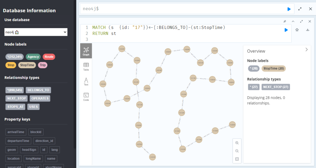
A prime example, are the relationships between GTFS StopTime and Trip nodes. For example, this is the Cypher query to get all StopTime nodes of Trip 17:

MATCH 
    (t:Trip  {id: "17"})
    <-[:BELONGS_TO]-
    (st:StopTime) 
RETURN st

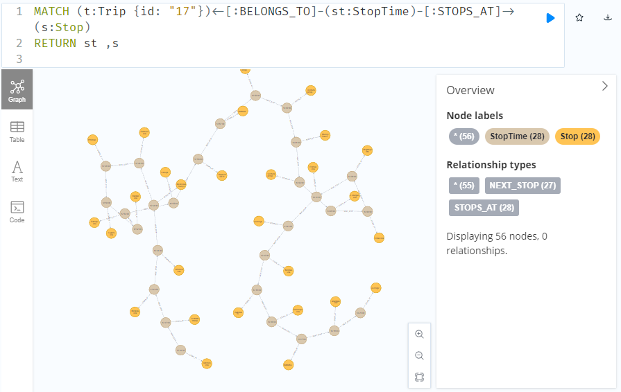
To get the stop locations, we also need to get the stop nodes:

MATCH 
    (t:Trip {id: "17"})
    <-[:BELONGS_TO]-
    (st:StopTime)
    -[:STOPS_AT]->
    (s:Stop)
RETURN st ,s

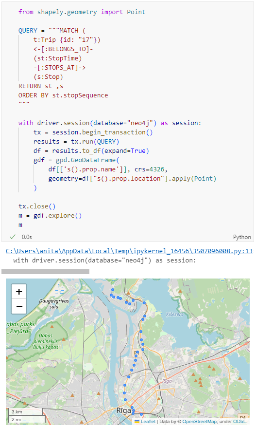
Adapting our code from the previous post, we can plot the stops:

from shapely.geometry import Point

QUERY = """MATCH (
    t:Trip {id: "17"})
    <-[:BELONGS_TO]-
    (st:StopTime)
    -[:STOPS_AT]->
    (s:Stop)
RETURN st ,s
ORDER BY st.stopSequence
"""

with driver.session(database="neo4j") as session:
    tx = session.begin_transaction()
    results = tx.run(QUERY)
    df = results.to_df(expand=True)
    gdf = gpd.GeoDataFrame(
        df[['s().prop.name']], crs=4326,
        geometry=df["s().prop.location"].apply(Point)
    )

tx.close() 
m = gdf.explore()
m

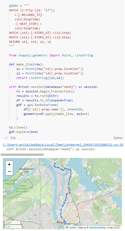
Ordering by stop sequence is actually completely optional. Technically, we could use the sorted GeoDataFrame, and aggregate all the points into a linestring to plot the route. But I want to try something different: we’ll use the NEXT_STOP relationships to get a DataFrame of the start and end stops for each segment:

QUERY = """
MATCH (t:Trip {id: "17"})
   <-[:BELONGS_TO]-
   (st1:StopTime)
   -[:NEXT_STOP]->
   (st2:StopTime)
MATCH (st1)-[:STOPS_AT]->(s1:Stop)
MATCH (st2)-[:STOPS_AT]->(s2:Stop)
RETURN st1, st2, s1, s2
"""

from shapely.geometry import Point, LineString

def make_line(row):
    s1 = Point(row["s1().prop.location"])
    s2 = Point(row["s2().prop.location"])
    return LineString([s1,s2])

with driver.session(database="neo4j") as session:
    tx = session.begin_transaction()
    results = tx.run(QUERY)
    df = results.to_df(expand=True)
    gdf = gpd.GeoDataFrame(
        df[['s1().prop.name']], crs=4326,
        geometry=df.apply(make_line, axis=1)
    )

tx.close() 
gdf.explore(m=m)

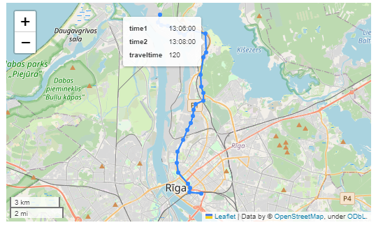
Finally, we can also use Cypher to calculate the travel time between two stops:

MATCH (t:Trip {id: "17"})
   <-[:BELONGS_TO]-
   (st1:StopTime)
   -[:NEXT_STOP]->
   (st2:StopTime)
MATCH (st1)-[:STOPS_AT]->(s1:Stop)
MATCH (st2)-[:STOPS_AT]->(s2:Stop)
RETURN st1.departureTime AS time1, 
   st2.arrivalTime AS time2, 
   s1.location AS geom1, 
   s2.location AS geom2, 
   duration.inSeconds(
      time(st1.departureTime), 
      time(st2.arrivalTime)
   ).seconds AS traveltime

As always, here’s the notebook: https://github.com/anitagraser/QGIS-resources/blob/master/qgis3/notebooks/neo4j.ipynb

Mapping Neo4j spatial nodes with GeoPandas

By underdark

2023-12-03

GIS, Movement data in GIS, Network, Visualization

In the recent post Setting up a graph db using GTFS data & Neo4J, we noted that — unfortunately — Neomap is not an option to visualize spatial nodes anymore.

GeoPandas to the rescue!

But first we need the neo4j Python driver:

pip install neo4j

Then we can connect to our database. The default user name is neo4j and you get to pick the password when creating the database:

from neo4j import GraphDatabase

URI = "neo4j://localhost"
AUTH = ("neo4j", "password")

with GraphDatabase.driver(URI, auth=AUTH) as driver:
    driver.verify_connectivity()

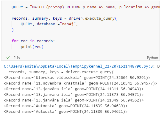
Once we have confirmed that the connection works as expected, we can run a query:

QUERY = "MATCH (p:Stop) RETURN p.name AS name, p.location AS geom"

records, summary, keys = driver.execute_query(
    QUERY, database_="neo4j",
)

for rec in records:
    print(rec)

Nice. There we have our GTFS stops, their names and their locations. But how to put them on a map?

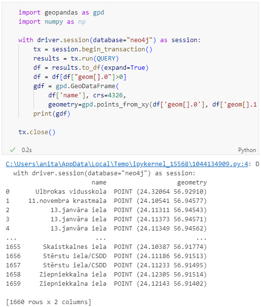
Conveniently, there is a to_db() function in the Neo4j driver:

import geopandas as gpd
import numpy as np

with driver.session(database="neo4j") as session:
    tx = session.begin_transaction()
    results = tx.run(QUERY)
    df = results.to_df(expand=True)
    df = df[df["geom[].0"]>0]
    gdf = gpd.GeoDataFrame(
        df['name'], crs=4326,
        geometry=gpd.points_from_xy(df['geom[].0'], df['geom[].1']))
    print(gdf)

tx.close()

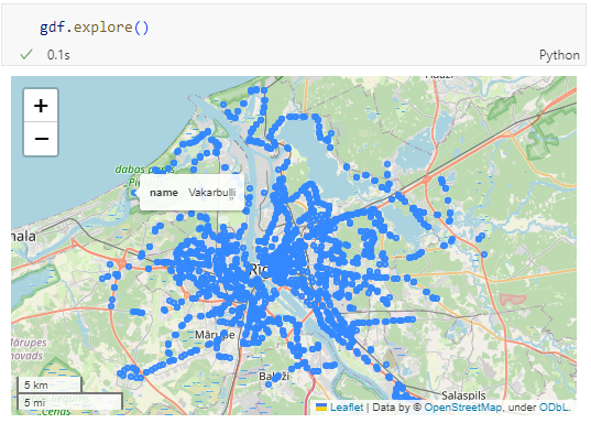
Since some of the nodes lack geometries, I added a quick and dirty hack to get rid of these nodes because — otherwise — gdf.explore() will complain about None geometries.

You can find this notebook at: https://github.com/anitagraser/QGIS-resources/blob/1e4ea435c9b1795ba5b170ddb176aa83689112eb/qgis3/notebooks/neo4j.ipynb

Next step will have to be the relationships. Stay posted.

Movement data in GIS #35: stop detection & analysis with MovingPandas

By underdark

2021-03-28

Data Mining, Movement data in GIS, MovingPandas

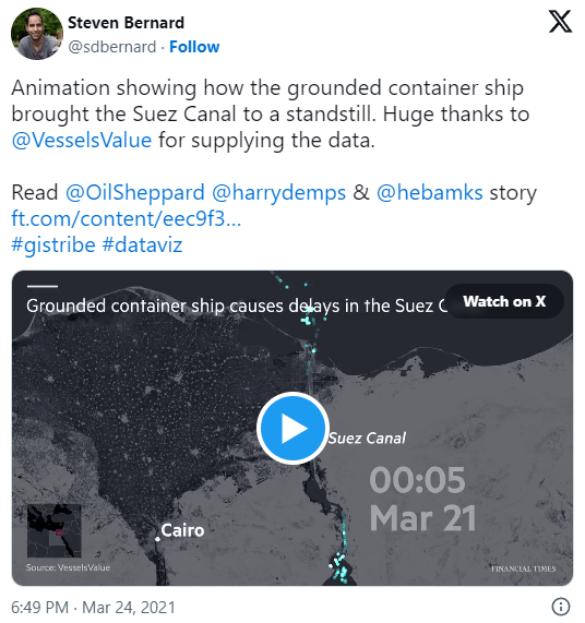
In the last few days, there’s been a sharp rise in interest in vessel movements, and particularly, in understanding where and why vessels stop. Following the grounding of Ever Given in the Suez Canal, satellite images and vessel tracking data (AIS) visualizations are everywhere:

Using movement data analytics tools, such as MovingPandas, we can dig deeper and explore patterns in the data.

The MovingPandas.TrajectoryStopDetector is particularly useful in this situation. We can provide it with a Trajectory or TrajectoryCollection and let it detect all stops, that is, instances were the moving object stayed within a certain area (with a diameter of 1000m in this example) for a an extended duration (at least 3 hours).

stops = mpd.TrajectoryStopDetector(trajs).get_stop_segments(
    min_duration=timedelta(hours=3), max_diameter=1000)

The resulting stop segments include spatial and temporal information about the stop location and duration. To make this info more easily accessible, let’s turn the stop segment TrajectoryCollection into a point GeoDataFrame:

stop_pts = gpd.GeoDataFrame(columns=['geometry']).set_geometry('geometry')
stop_pts['stop_id'] = [track.id for track in stops.trajectories]
stop_pts= stop_pts.set_index('stop_id')

for stop in stops:
    stop_pts.at[stop.id, 'ID'] = stop.df['ID'][0]
    stop_pts.at[stop.id, 'datetime'] = stop.get_start_time()
    stop_pts.at[stop.id, 'duration_h'] = stop.get_duration().total_seconds()/3600
    stop_pts.at[stop.id, 'geometry'] = stop.get_start_location()

Indeed, I think the next version of MovingPandas should include a function that directly returns stops as points.

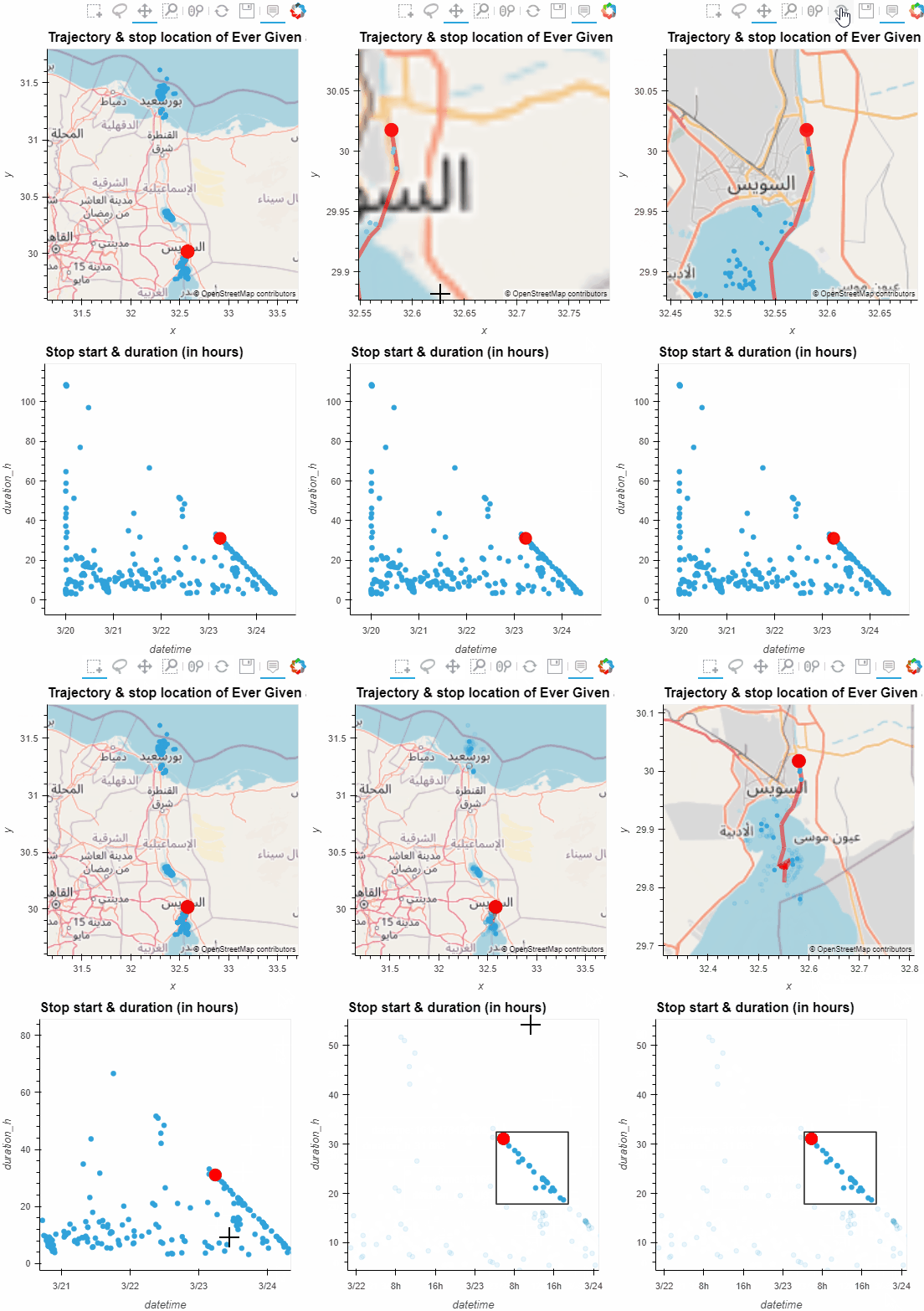
Now we can explore the stop information. For example, the map plot shows that stops are concentrated in three main areas: the northern and southern ends of the Canal, as well as the Great Bitter Lake in the middle. By looking at the timing of stops and their duration in a scatter plot, we can clearly see that the Ever Given stop (red) caused a chain reaction: the numerous points lining up on the diagonal of the scatter plot represent stops that very likely are results of the blockage:

Before the grounding, the stop distribution nicely illustrates the canal schedule. Vessels have to wait until it’s turn for their direction to go through:

You can see the full analysis workflow in the following video. Please turn on the captions for details.

Huge thanks to VesselsValue for supplying the data!

For another example of MovingPandas‘ stop dectection in action, have a look at Bryan R. Vallejo’s tutorial on detecting stops in bird tracking data which includes some awesome visualizations using KeplerGL:

Kepler.GL visualization by Bryan R. Vallejo

This post is part of a series. Read more about movement data in GIS.

Introducing the open data analysis OGD.AT Lab

By underdark

2021-02-11

GIS

Data sourcing and preparation is one of the most time consuming tasks in many spatial analyses. Even though the Austrian data.gv.at platform already provides a central catalog, the individual datasets still vary considerably in their accessibility or readiness for use.

OGD.AT Lab is a new repository collecting Jupyter notebooks for working with Austrian Open Government Data and other auxiliary open data sources. The notebooks illustrate different use cases, including so far:

Accessing geodata from the city of Vienna WFS
Downloading environmental data (heat vulnerability and air quality)
Geocoding addresses and getting elevation information
Exploring urban movement data

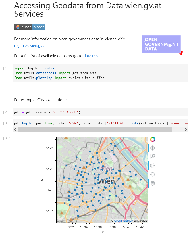
Data processing and visualization are performed using Pandas, GeoPandas, and Holoviews. GeoPandas makes it straighforward to use data from WFS. Therefore, OGD.AT Lab can provide one universal gdf_from_wfs() function which takes the desired WFS layer as an argument and returns a GeoPandas.GeoDataFrame that is ready for analysis:

Launch this notebook in: https://mybinder.org/v2/gh/anitagraser/ogd-at-lab/v0.1?urlpath=lab/tree/notebooks/wien-ogd.ipynb

Many other datasets are provided as CSV files which need to be joined with spatial datasets to use them in spatial analysis. For example, the “Urban heat vulnerability index” dataset which needs to be joined to statistical areas.

Launch this notebook in Mybinder: https://mybinder.org/v2/gh/anitagraser/ogd-at-lab/v0.1?urlpath=lab/tree/notebooks/environment.ipynb

Another issue with many CSV files is that they use German number formatting, where commas are used as a decimal separater instead of dots:

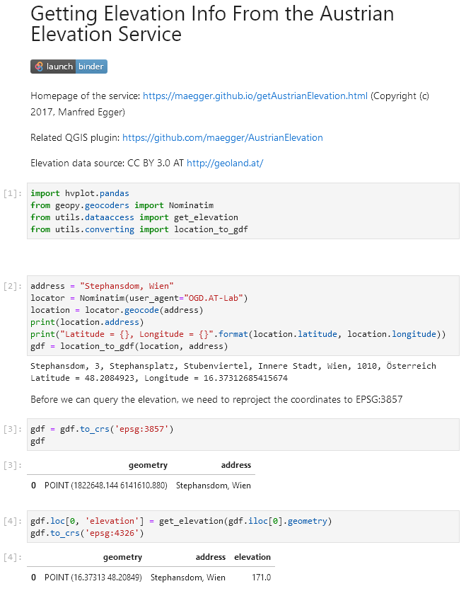
Besides file access, there are also open services provided by other developers, for example, Manfred Egger developed an elevation service that provides elevation information for any point in Austria. In combination with geocoding services, such as Nominatim, this makes is possible to, for example, find the elevation for any address in Austria:

Launch this notebook in MyBinder: https://mybinder.org/v2/gh/anitagraser/ogd-at-lab/v0.1?urlpath=lab/tree/notebooks/elevation.ipynb

Last but not least, the first version of the mobility notebook showcases open travel time data provided by Uber Movement:

Launch this notebook in Mybinder: https://mybinder.org/v2/gh/anitagraser/ogd-at-lab/v0.1?urlpath=lab/tree/notebooks/mobility.ipynb

The utility functions for data access included in this repository will continue to grow as new data sources are included. Eventually, it may make sense to extract the data access function into a dedicated library, similar to geofi (Finland) or geobr (Brazil).

If you’re aware of any interesting open datasets or services that should be included in OGD.AT, feel free to reach out here or on Github through the issue tracker or by providing a pull request.