Archive

Tag Archives: OSM

Wrong navigation instructions can be annoying and sometimes even dangerous, but they happen. No dataset is free of errors. That’s why it’s important to assess the quality of datasets. One specific use case I previously presented at FOSS4G 2013 is the quality assessment of turn restrictions in OSM, which influence vehicle routing results.

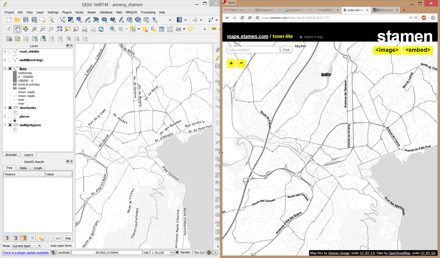
The main idea is to compare OSM to another data source. For this example, I used turn restriction data from the City of Toronto. Of the more than 70,000 features in this dataset, I extracted a sample of about 500 turn restrictions around Ryerson University, which I had the pleasure of visiting in 2014.

As you can see from the following screenshot, OSM and the city’s dataset agree on 420 of 504 restrictions (83%), while 36 cases (7%) are in clear disagreement. The remaining cases require further visual inspection.

toronto_turns_overview

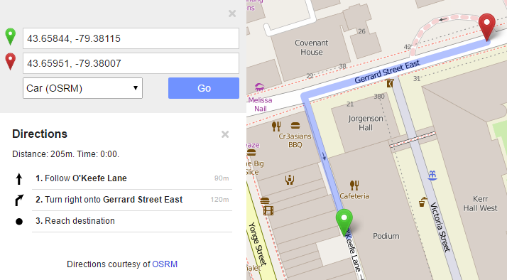
The following two examples show one case where the turn restriction is modelled in both datasets (on the left) and one case where OSM does not agree with the city data (on the right).
In the first case, the turn restriction (short green arrow) tells us that cars are not allowed to turn right at this location. An OSM-based router (here I used OpenRouteService.org) therefore finds a route (blue dashed arrow) which avoids the forbidden turn. In the second case, the router does not avoid the forbidden turn. We have to conclude that one of the two datasets is wrong.

If you want to learn more about the methodology, please check Graser, A., Straub, M., & Dragaschnig, M. (2014). Towards an open source analysis toolbox for street network comparison: indicators, tools and results of a comparison of OSM and the official Austrian reference graph. Transactions in GIS, 18(4), 510-526. doi:10.1111/tgis.12061.

Interestingly, the disagreement in the second example has been fixed by a recent edit (only 14 hours ago). We can see this in the OSM way history, which reveals that the line direction has been switched, but this change hasn’t made it into the routing databases yet:

This leads to the funny situation that the oneway is correctly displayed on the map but seemingly ignored by the routers:

toronto_okeefe_osrm

To evaluate the results of the automatic analysis, I wrote a QGIS script, which allows me to step through the results and visually compare turn restrictions and routing results. It provides a function called next() which updates a project variable called myvar. This project variable controls which features (i.e. turn restriction and associated route) are rendered. Finally, the script zooms to the route feature:

def next():
    f = features.next()
    id = f['TURN_ID']
    print "Going to %s" % (id)
    QgsExpressionContextUtils.setProjectVariable('myvar',id)
    iface.mapCanvas().zoomToFeatureExtent(f.geometry().boundingBox())
    if iface.mapCanvas().scale() < 500:
        iface.mapCanvas().zoomScale(500)

layer = iface.activeLayer()
features = layer.getFeatures()
next()

You can see it in action here:

I’d love to see this as an interactive web map where users can have a look at all results, compare with other routing services – or ideally the real world – and finally fix OSM where necessary.

This work has been in the making for a while. I’d like to thank the team of OpenRouteService.org who’s routing service I used (and who recently added support for North America) as well as my colleagues at Ryerson University in Toronto, who pointed me towards Toronto’s open data.

Advertisement

It’s my pleasure to report back from this year’s AGIT and GI_Forum conference (German and English speaking respectively). It was great to meet the gathered GIS crowd! If you missed it, don’t despair: I’ve compiled a personal summary on Storify, and papers (German, English) and posters are available online. Here’s a pick of my favorite posters:

I also had the pleasure to be involved in multiple presentations this year:

QGIS at the OSGeo Day

As part of the OSGeo Day, I had the chance to present the latest and greatest QGIS features for map design in front of a full house:

Routing with OSM

On a slightly different note, my colleague Markus Straub and I presented an introduction to routing with OpenStreetMap covering which kind of routing-related information is available in OSM as well as a selection of different tools to perform routing on OSM.

Solving the “unnamed link” problem

In this talk, I presented approaches to solving issues with route descriptions that contain unnamed pedestrian or cycle paths.

Here you can find the full open access paper: Graser, A., & Straub, M. (2015). Improving Navigation: Automated Name Extraction for Separately Mapped Pedestrian and Cycle Links. GI_Forum ‒ Journal for Geographic Information Science, 1-2015, 546-556, doi:10.1553/giscience2015s546.

Inferring road popularity from GPS trajectories

In this talk, my colleague Markus Straub presented our new approach to computing how popular a certain road is. The resulting popularity value can be used for planning as well as routing.

Here you can find the full open access paper: Straub, M., & Graser, A. (2015). Learning from Experts: Inferring Road Popularity from GPS Trajectories. GI_Forum ‒ Journal for Geographic Information Science, 1-2015, 41-50, doi:10.1553/giscience2015s41.

How do you objectively define and compute which parts of a network are in the center? One approach is to use the concept of centrality.

Centrality refers to indicators which identify the most important vertices within a graph. Applications include identifying the most influential person(s) in a social network, key infrastructure nodes in the Internet or urban networks, and super spreaders of disease. (Source: http://en.wikipedia.org/wiki/Centrality)

Researching this topic, it turns out that some centrality measures have already been implemented in GRASS GIS. thumbs up!

v.net.centrality computes degree, betweeness, closeness and eigenvector centrality.

As a test, I’ve loaded the OSM street network of Vienna and run

v.net.centrality -a input=streets@anita_000 output=centrality degree=degree closeness=closeness betweenness=betweenness eigenvector=eigenvector

grass_centrality

The computations take a while.

In my opinion, the most interesting centrality measures for this street network are closeness and betweenness:

Closeness “measures to which extent a node i is near to all the other nodes along the shortest paths”. Closeness values are lowest in the center of the network and higher in the outskirts.

Betweenness “is based on the idea that a node is central if it lies between many other nodes, in the sense that it is traversed by many of the shortest paths connecting couples of nodes.” Betweenness values are highest on bridges and other important arterials while they are lowest for dead-end streets.

(Definitions as described in more detail in Crucitti, Paolo, Vito Latora, and Sergio Porta. “Centrality measures in spatial networks of urban streets.” Physical Review E 73.3 (2006): 036125.)

Centrality: low values in pink, high values in green

Centrality: low values in pink, high values in green

Works great! Unfortunately, v.net.centrality is not yet part of the QGIS Processing GRASS toolbox. It would certainly be a great addition.

Correct turn restriction information is essential for the vehicle routing quality of any street network dataset – open or commercial. One of the challenges of this kind of information is that these restrictions are typically not directly visible on each map.

This post is inspired by a share on G+ which resurfaced in my notifications. In a post on the Mapbox blog, John Firebaugh presents the OSM iD editor which should make editing turn restrictions straight-forward: clicking on the source link turns the associated turn information visible. By clicking on the turn arrows, the user can easily toggle between allowed and forbidden.

iD, the web editor for OpenStreetMap, makes it even simpler to add turn restrictions to OpenStreetMap.

editing turn restrictions in iD, the web editor for OpenStreetMap. source: “Simple Editing for Turn Restrictions in OpenStreetMap” by John Firebaugh on June 06 2014

But the issue of identifying wrong turn restrictions remains. One approach to solving this issue is to compare restriction information in OSM with the information in a reference data set.

This is possible by comparing routes computed on OSM and the reference data using a method I presented at FOSS4G (video): a turn restriction basically is a forbidden combination of links. If we compute the route from the start link of the forbidden combination to the end link, we can check if the resulting route geometry violates the restriction or uses an appropriate detour:

read more about this method and results:

illustrative slide from my LBS2014 presentation on OSM vehicle routing quality – read more about this method and results for Vienna in our TGIS paper or the open pre-print version

It would be great to have an automated system comparing OSM and open government street network data to detect these differences. The quality of both data sets could benefit enormously by bundling their QA efforts. Unfortunately, the open government street network data sets I’m aware of don’t contain turn information.

In my opinion, Stamen’s Toner-lite map is one of the best background maps to use together with colorful overlays. The only downsides of using it in QGIS are that the OpenLayers plugin can not provide the tiles at print resolution and that the projection is limited to Web Mercator. That’s why I’ve started to recreate the style for OSM Spatialite databases:

toner-lite

So far, there are styles for lines and polygons and they work quite well for the scale range between 1:1 and 1:250000. As always, you can download the styles from QGIS-resources on Github.

Using OSM data in QGIS is a hot topic but so far, no best practices for downloading, preprocessing and styling the data have been established. There are many potential solutions with all their advantages and disadvantages. To give you a place to start, I thought I’d share a workflow which works for me to create maps like the following one from nothing but OSM:

osm_google_100k

Getting the data

Raw OSM files can be quite huge. That’s why it’s definitely preferable to download the compressed binary .pbf format instead of the XML .osm format.

As a download source, I’d recommend Geofabrik. The area in the example used in this post is part of the region Pays de la Loire, France.

Preparing the data for QGIS

In the preprocessing step, we will extract our area of interest and convert the .pbf into a spatialite database which can be used directly in QGIS.

This can be done in one step using ogr2ogr:

C:\Users\anita_000\Geodata\OSM_Noirmoutier>ogr2ogr -f "SQLite" -dsco SPATIALITE=YES -spat 2.59 46.58 -1.44 47.07 noirmoutier.db noirmoutier.pbf

where the -spat option controls the area of interest to be extracted.

When I first published this post, I suggested a two step approach. You can find it here for future reference:

For the first step: extracting the area of interest, we need Osmosis. (For Windows, you can get osmosis from openstreetmap.org. Unpack to use. Requires Java.)

When you have Osmosis ready, we can extract the area of interest to the .osm format:

C:\Users\anita_000\Geodata\OSM_Noirmoutier>..\bin\osmosis.bat --read-pbf pays-de-la-loire-latest.osm.pbf --bounding-box left=-2.59 bottom=46.58 right=-1.44 top=47.07 --write-xml noirmoutier.osm

While QGIS can also load .osm files, I found that performance and access to attributes is much improved if the .osm file is converted to spatialite. Luckily, that’s easy using ogr2ogr:

C:\Users\anita_000\Geodata\OSM_Noirmoutier>ogr2ogr -f "SQLite" -dsco SPATIALITE=YES noirmoutier.db noirmoutier.osm

Finishing preprocessing in QGIS

In QGIS, we’ll want to load the points, lines, and multipolygons using Add SpatiaLite Layer:

Screenshot 2014-05-31 11.39.40

When we load the spatialite tables, there are a lot of features and some issues:

  • There is no land polygon. Instead, there are “coastline” line features.
  • Most river polygons are missing. Instead there are “riverbank” line features.

Screenshot 2014-05-31 11.59.58

Luckily, creating the missing river polygons is not a big deal:

  1. First, we need to select all the lines where waterway=riverbank.
    Screenshot 2014-05-31 13.14.00
  2. Then, we can use the Polygonize tool from the processing toolbox to automatically create polygons from the areas enclosed by the selected riverbank lines. (Note that Processing by default operates only on the selected features but this setting can be changed in the Processing settings.)
    Screenshot 2014-05-31 13.40.16

Creating the land polygon (or sea polygon if you prefer that for some reason) is a little more involved since most of the time the coastline will not be closed for the simple reason that we are often cutting a piece of land out of the main continent. Therefore, before we can use the Polygonize tools, we have to close the area. To do that, I suggest to first select the coastline using "other_tags" LIKE '%"natural"=>"coastline"%' and create a new layer from this selection (save selection as …) and edit it (don’t forget to enable snapping!) to add lines to close the area. Then polygonize.

Screenshot 2014-05-31 14.38.48

Styling the data

Now that all preprocessing is done, we can focus on the styling.

You can get the styles used in the map from my Github QGIS-resources repository:

  • osm_spatialite_googlemaps_multipolygon.qml … rule-based renderer incl. rules for: water, natural, residential areas and airports
  • osm_spatialite_googlemaps_lines.qml … rule-based renderer incl. rules for roads, rails, and rivers, as well as rules for labels
  • osm_spatialite_googlemaps_roadshields.qml … special label style for road shields
  • osm_spatialite_googlemaps_places.qml … label style for populated places such as cities and towns

qgis_osm_google_100k

Extracting POIs from OpenStreetMap is reasonably simple using Overpass API. A very convenient way to construct the query is to use a query builder which allows you to select the area of interest and builds queries for different servers.

xapi_query_builder

Of course you can fine-tune the query further. For example, you can add multiple key-value pairs to the query. I used the following query to select all Billa supermarkets:

www.overpass-api.de/api/xapi?*[shop=supermarket][name=Billa][bbox=15.96725,48.0432,16.79947,48.40915]

Note the * in the query? It means that I’m querying all kinds of features: nodes, ways, and relations.

Save the server response to a .osm file. This file can be loaded into QGIS using simple drag-and-drop or Add Vector Layer. A dialog will open where you can select the type of features you want to load from the file. You can simply use Select All and OK to load everything.

add_osm_file

My supermarket POIs came in two types: points and multipolygons. To style them both with nice supermarket SVG icons, I decided to use a Centroid fill with the SVG marker for the polygon layer:

osm_pois_billa

Open data and open source GIS … nice :-)

OSM place search and osmSearch are two plugins for QGIS which use the Nominatim service to find addresses and places. They are both still marked as “experimental” plugins, so users are expected to expect the unexpected.

Once installed, both plugins look very similar: There is an input text field and a results list.

osmsearch_giefinggasse

A simple search with street name and house number returns the expected results. Interacting with the result shows some differences:

  • OSM place search will highlight the location when you mouse-over the result in the list. On double-click, it will zoom to the result.
  • osmSearch will highlight the result and move the map center to the result if you double-click but won’t zoom.

Both plugins can deal with umlauts (ä,ö,ü) but only osmSearch works with háčeks.

osmsearch_hacek

A nice feature of osmSearch is that it remembers your previous searches and offers an auto-complete function.

OSM place search on the other hand offers a reverse “Where am I” function (the arrow pointing to the left” which tries to find a name for the current map center location. Additionally, there are functions to add the current object as a new layer or mask layer.

Both plugins have strong and weak points. Combined, they would make a really strong tool but then nothing prevents us from having them both and choosing the best one for the task at hand.

In my previous post, I presented a Processing model to determine positional accuracy of street networks. Today, I’ll cover another very popular tool to assess OSM quality in a region: network length comparison. Here’s the corresponding slide from my FOSS4G presentation which shows an example of this approach applied to OSM and OS data in the UK:

foss4g_osm_data_quality_12

One building block of this tool is the Total graph length model which calculates the length of a network within specified regions. Like the model for positional accuracy, this model includes reprojection steps to ensure all layers are in the same CRS before the actual geoprocessing starts:

total_graph_length

The final Compare total graph length model combines two instances of “Total graph length” whose results are then joined to eventually calculate the length difference (lenDIFF).

compare_total_graph_length

As usual, you can find the models on Github. If you have any questions, don’t hesitate to ask in the comments and if you find any issues please report them on Github.

Please read the new instructions for QGIS 2.

I’ve added a new style for osm2po layers to the QGIS Resources Github repo. It contains the following rules:

the rules

and looks like this:

the map

Enjoy!

%d bloggers like this: