Analyzing video-based bicycle trajectories
Did you know that MovingPandas also supports local image coordinates? Indeed, it does.
In today’s post, we will explore how we can use this feature to analyze bicycle tracks extracted from video footage published by Michael Szell @mszll:
- Dataset: https://zenodo.org/record/7288616
- Data description: https://arxiv.org/abs/2211.01301
The bicycle trajectory coordinates are stored in two separate lists: xs_640x360 and ys640x360:
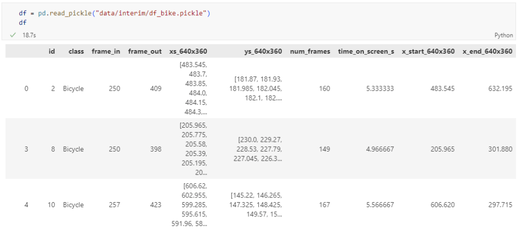
This format is kind of similar to the Kaggle Taxi dataset, we worked with in the previous post. However, to use the solution we implemented there, we need to combine the x and y coordinates into nice (x,y) tuples:
df['coordinates'] = df.apply(
    lambda row: list(zip(row['xs_640x360'], row['ys_640x360'])), axis=1)
df.drop(columns=['xs_640x360', 'ys_640x360'], inplace=True)
Afterwards, we can create the points and compute the proper timestamps from the frame numbers:
def compute_datetime(row):
    # some educated guessing going on here: the paper states that the video covers 2021-06-09 07:00-08:00
    d = datetime(2021,6,9,7,0,0) + (row['frame_in'] + row['running_number']) * timedelta(seconds=2)
    return d
def create_point(xy):
    try:
        return Point(xy)
    except TypeError:  # when there are nan values in the input data
        return None
new_df = df.head().explode('coordinates')
new_df['geometry'] = new_df['coordinates'].apply(create_point)
new_df['running_number'] = new_df.groupby('id').cumcount()
new_df['datetime'] = new_df.apply(compute_datetime, axis=1)
new_df.drop(columns=['coordinates', 'frame_in', 'running_number'], inplace=True)
new_df
Once the points and timestamps are ready, we can create the MovingPandas TrajectoryCollection. Note how we explicitly state that there is no CRS for this dataset (crs=None):
trajs = mpd.TrajectoryCollection(
    gpd.GeoDataFrame(new_df),
    traj_id_col='id',  t='datetime', crs=None)
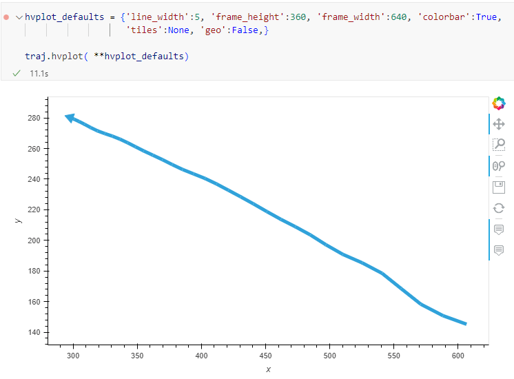
Plotting trajectories with image coordinates
Similarly, to plot these trajectories, we should tell hvplot that it should not fetch any background map tiles (’tiles’:None) and that the coordinates are not geographic (‘geo’:False):
If you want to explore the full source code, you can find my Github fork with the Jupyter notebook at: https://github.com/anitagraser/desirelines/blob/main/mpd.ipynb
The repository also contains a camera image of the intersection, which we can use as a background for our trajectory plots:
bg_img = hv.RGB.load_image('img/intersection2.png', bounds=(0,0,640,360))
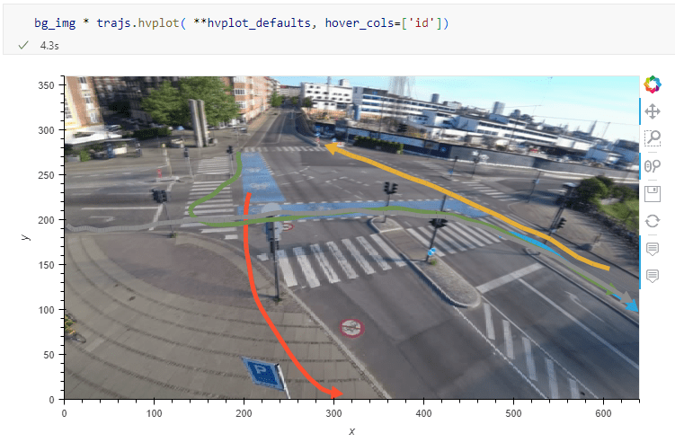
One important caveat is that speed will be calculated in pixels per second. So when we plot the bicycle speed, the segments closer to the camera will appear faster than the segments in the background:

To fix this issue, we would have to correct for the distortions of the camera lens and perspective. I’m sure that there is specialized software for this task but, for the purpose of this post, I’m going to grab the opportunity to finally test out the VectorBender plugin.
Georeferencing the trajectories using QGIS VectorBender plugin
Let’s load the five test trajectories and the camera image to QGIS. To make sure that they align properly, both are set to the same CRS and I’ve created the following basic world file for the camera image:
1
0
0
-1
0
360
Then we can use the VectorBender tools to georeference the trajectories by linking locations from the camera image to locations on aerial images. You can see the whole process in action here:
After around 15 minutes linking control points, VectorBender comes up with the following georeferenced trajectory result:
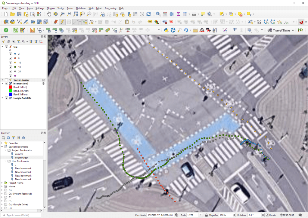
Not bad for a quick-and-dirty hack. Some points on the borders of the image could not be georeferenced since I wasn’t always able to identify suitable control points at the camera image borders. So it won’t be perfect but should improve speed estimates.
This post is part of a series. Read more about movement data in GIS.

Hi Anita, which CRS was used for the camera image and the first five trajectories?
Hi Song. I assigned Web Mercator to all layers in the project in order to avoid potential sources of confusion for the Vector Bender plugin.
Hi Anita, after I set EPSG:3857 for all layers (google map, 5 trajs, camera image, and vector bender), the preview button of vector bender plugin works fine, but the final result does not appear. What are the possible reasons? I am using QGIS3.18, and my google map is https://www.google.cn/maps/vt?lyrs=s@189&gl=cn&x={x}&y={y}&z={z}
Oh, it works now. The reason seems to be that I saved the 5trajs as geojson format before (without specified EPSG:3857) and set EPSG:3587 in QGIS. Now I save the 5 trajs again as a shapefile and also the EPSG:3857 information in this shapefile. Thanks!
That’s great to hear. Thank you for sharing the details of your workflow.