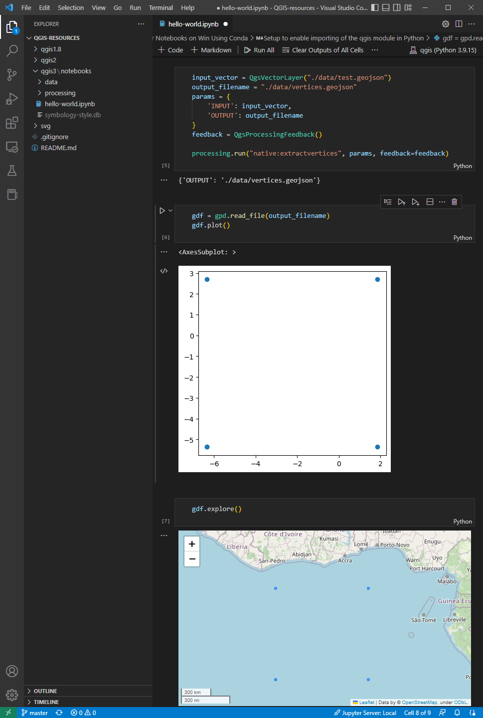
Earlier this year, we explored how to use PyQGIS in Juypter notebooks to run QGIS Processing tools from a notebook and visualize the Processing results using GeoPandas plots.
Today, we’ll go a step further and replace the GeoPandas plots with maps rendered by QGIS.
The following script presents a minimum solution to this challenge: initializing a QGIS application, canvas, and project; then loading a GeoJSON and displaying it:
from IPython.display import Image

from PyQt5.QtGui import QColor
from PyQt5.QtWidgets import QApplication

from qgis.core import QgsApplication, QgsVectorLayer, QgsProject, QgsSymbol, \
    QgsRendererRange, QgsGraduatedSymbolRenderer, \
    QgsArrowSymbolLayer, QgsLineSymbol, QgsSingleSymbolRenderer, \
    QgsSymbolLayer, QgsProperty
from qgis.gui import QgsMapCanvas

app = QApplication([])
qgs = QgsApplication([], False)
canvas = QgsMapCanvas()
project = QgsProject.instance()

vlayer = QgsVectorLayer("./data/traj.geojson", "My trajectory")
if not vlayer.isValid():
    print("Layer failed to load!")

def saveImage(path, show=True):
    canvas.saveAsImage(path)
    if show: return Image(path)

project.addMapLayer(vlayer)
canvas.setExtent(vlayer.extent())
canvas.setLayers([vlayer])
canvas.show()
app.exec_()

saveImage("my-traj.png")
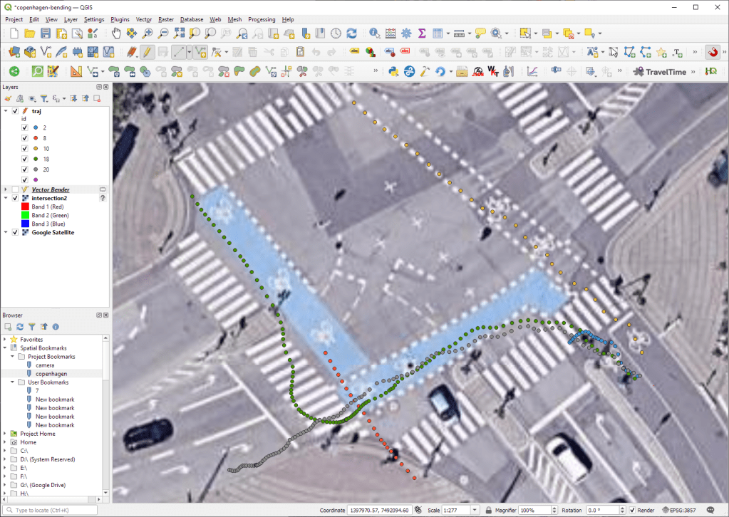
When this code is executed, it opens a separate window that displays the map canvas. And in this window, we can even pan and zoom to adjust the map. The line color, however, is assigned randomly (like when we open a new layer in QGIS):

To specify a specific color, we can use:
vlayer.renderer().symbol().setColor(QColor("red"))

vlayer.triggerRepaint()
canvas.show()
app.exec_()
saveImage("my-traj.png")

But regular lines are boring. We could easily create those with GeoPandas plots.
Things get way more interesting when we use QGIS’ custom symbols and renderers. For example, to draw arrows using a QgsArrowSymbolLayer, we can write:
vlayer.renderer().symbol().appendSymbolLayer(QgsArrowSymbolLayer())

vlayer.triggerRepaint()
canvas.show()
app.exec_()
saveImage("my-traj.png")

We can also create a QgsGraduatedSymbolRenderer:
geom_type = vlayer.geometryType()
myRangeList = []

symbol = QgsSymbol.defaultSymbol(geom_type)
symbol.setColor(QColor("#3333ff"))
myRange = QgsRendererRange(0, 1, symbol, 'Group 1')
myRangeList.append(myRange)

symbol = QgsSymbol.defaultSymbol(geom_type)
symbol.setColor(QColor("#33ff33"))
myRange = QgsRendererRange(1, 3, symbol, 'Group 2')
myRangeList.append(myRange)

myRenderer = QgsGraduatedSymbolRenderer('speed', myRangeList)
vlayer.setRenderer(myRenderer)

vlayer.triggerRepaint()
canvas.show()
app.exec_()
saveImage("my-traj.png")

And we can combine both QgsGraduatedSymbolRenderer and QgsArrowSymbolLayer:
geom_type = vlayer.geometryType()
myRangeList = []

symbol = QgsSymbol.defaultSymbol(geom_type)
symbol.appendSymbolLayer(QgsArrowSymbolLayer())
symbol.setColor(QColor("#3333ff"))
myRange = QgsRendererRange(0, 1, symbol, 'Group 1')
myRangeList.append(myRange)

symbol = QgsSymbol.defaultSymbol(geom_type)
symbol.appendSymbolLayer(QgsArrowSymbolLayer())
symbol.setColor(QColor("#33ff33"))
myRange = QgsRendererRange(1, 3, symbol, 'Group 2')
myRangeList.append(myRange)

myRenderer = QgsGraduatedSymbolRenderer('speed', myRangeList)
vlayer.setRenderer(myRenderer)

vlayer.triggerRepaint()
canvas.show()
app.exec_()
saveImage("my-traj.png")

Maybe the most powerful option is to use data-defined symbology. For example, to control line width and color:
renderer = QgsSingleSymbolRenderer(QgsSymbol.defaultSymbol(geom_type))

exp_width = 'scale_linear("speed", 0, 3, 0, 7)'
exp_color = "coalesce(ramp_color('Viridis',scale_linear(\"speed\", 0, 3, 0, 1)), '#000000')"

# https://qgis.org/pyqgis/3.0/core/Symbol/QgsSymbolLayer.html?highlight=property#qgis.core.QgsSymbolLayer.PropertySize
renderer.symbol().symbolLayer(0).setDataDefinedProperty(
    QgsSymbolLayer.PropertyStrokeWidth, QgsProperty.fromExpression(exp_width))
renderer.symbol().symbolLayer(0).setDataDefinedProperty(
    QgsSymbolLayer.PropertyStrokeColor, QgsProperty.fromExpression(exp_color))
renderer.symbol().symbolLayer(0).setDataDefinedProperty(
    QgsSymbolLayer.PropertyCapStyle, QgsProperty.fromExpression("'round'"))

vlayer.setRenderer(renderer)

vlayer.triggerRepaint()
canvas.show()
app.exec_()
saveImage("my-traj.png")

Find the full notebook at: https://github.com/anitagraser/QGIS-resources/blob/master/qgis3/notebooks/layer-styling.ipynb