Many of you certainly have already heard of and/or even used Leafmap by Qiusheng Wu.

Leafmap is a Python package for interactive spatial analysis with minimal coding in Jupyter environments. It provides interactive maps based on folium and ipyleaflet, spatial analysis functions using WhiteboxTools and whiteboxgui, and additional GUI elements based on ipywidgets.

This way, Leafmap achieves a look and feel that is reminiscent of a desktop GIS:

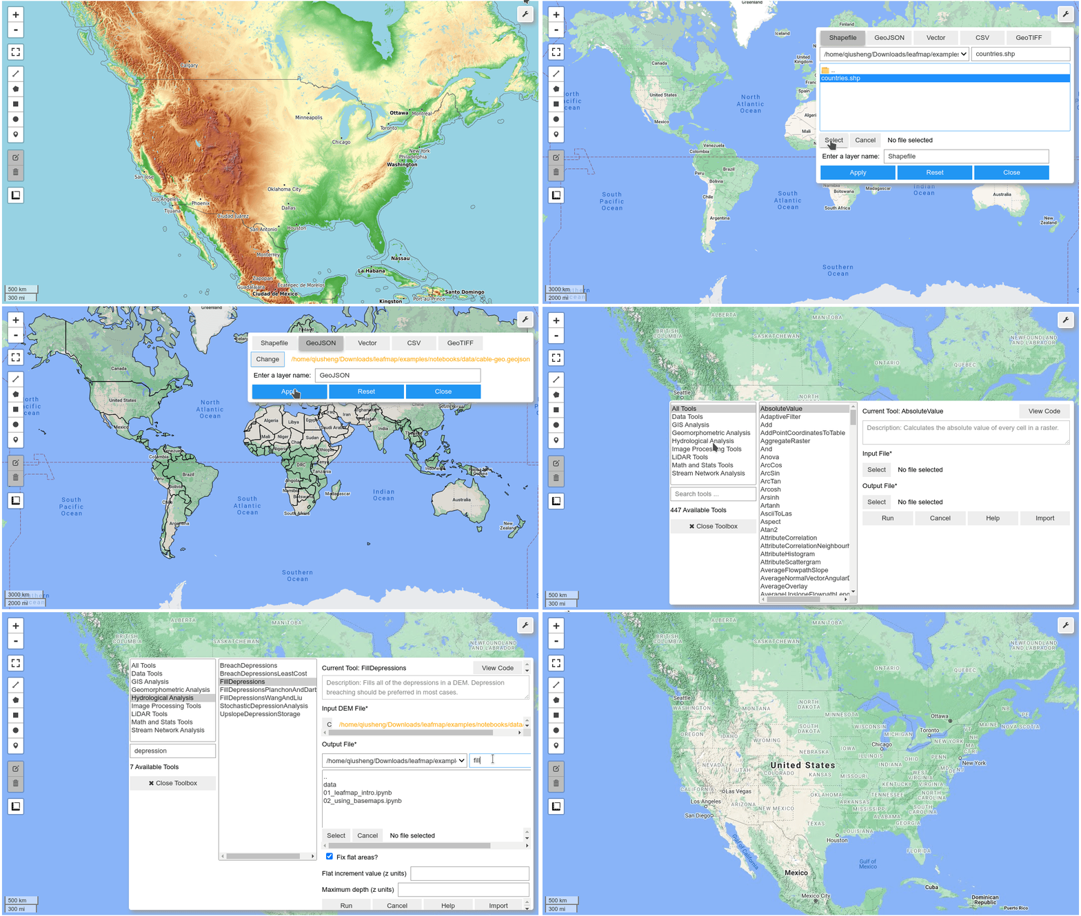
Image source: https://github.com/giswqs/leafmap

Recently, Qiusheng has started an additional project: the geospatial meta package which brings together a variety of different Python packages for geospatial analysis. As such, the main goals of geospatial are to make it easier to discover and use the diverse packages that make up the spatial Python ecosystem.

Besides the usual suspects, such as GeoPandas and of course Leafmap, one of the packages included in geospatial is MovingPandas. Thanks, Qiusheng!

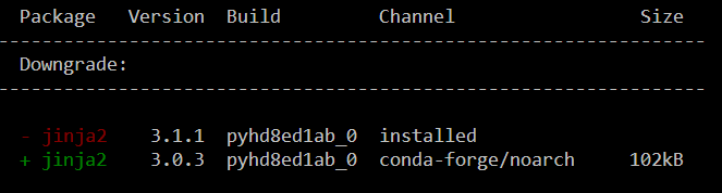
I’ve tested the mamba install today and am very happy with how this worked out. There is just one small hiccup currently, which is related to an upstream jinja2 issue. After installing geospatial, I therefore downgraded jinja:

mamba install -c conda-forge geospatial 
mamba install -c conda-forge jinja2=3.0

Of course, I had to try Leafmap and MovingPandas in action together. Therefore, I fired up one of the MovingPandas example notebook (here the example on clipping trajectories using polygons). As you can see, the integration is pretty smooth since Leafmap already support drawing GeoPandas GeoDataFrames and MovingPandas can convert trajectories to GeoDataFrames (both lines and points):

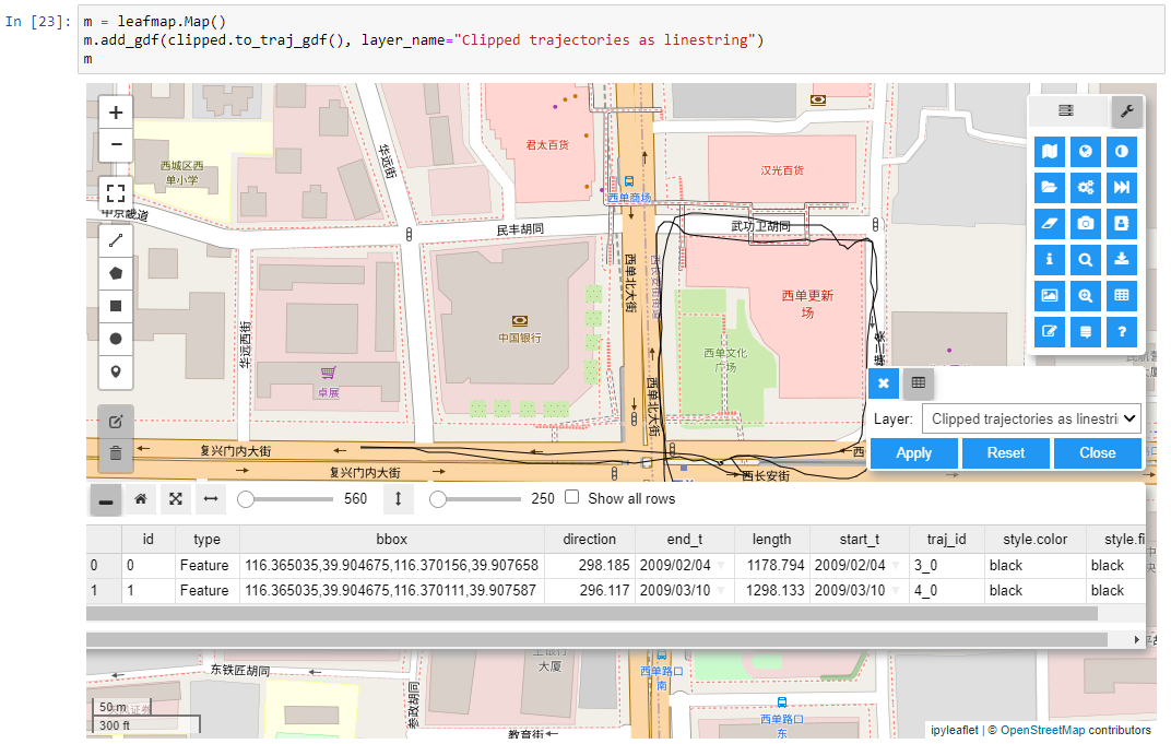
Clipped trajectory segments as linestrings in Leafmap

Leafmap includes an attribute table view that can be activated on user request to show, e.g. trajectory information

And, of course, we can also map the original trajectory points

Geospatial also includes the new dask-geopandas library which I’m very much looking forward to trying out next.

MovingPandas now supports local coordinates

By underdark

2022-03-06

MovingPandas, spatio-temporal data

MovingPandas 0.9rc3 has just been released, including important fixes for local coordinate support. Sports analytics is just one example of movement data analysis that uses local rather than geographic coordinates.

Many movement data sources – such as soccer players’ movements extracted from video footage – use local reference systems. This means that x and y represent positions within an arbitrary frame, such as a soccer field.

Since Geopandas and GeoViews support handling and plotting local coordinates just fine, there is nothing stopping us from applying all MovingPandas functionality to this data. For example, to visualize the movement speed of players:

Of course, we can also plot other trajectory attributes, such as the team affiliation.

But one particularly useful feature is the ability to use custom background images, for example, to show the soccer field layout:

To access the full example notebook, visit: https://github.com/anitagraser/movingpandas/blob/master/tutorials/5-local-coordinates.ipynb

An update to the MovingPandas examples repository will follow shortly.

This post is part of a series. Read more about movement data in GIS.

MovingPandas v0.9 released!

By underdark

2022-01-15

MovingPandas

1 Comment

The latest v0.9 release is now available from conda-forge.

This release contains some really cool new algorithms:

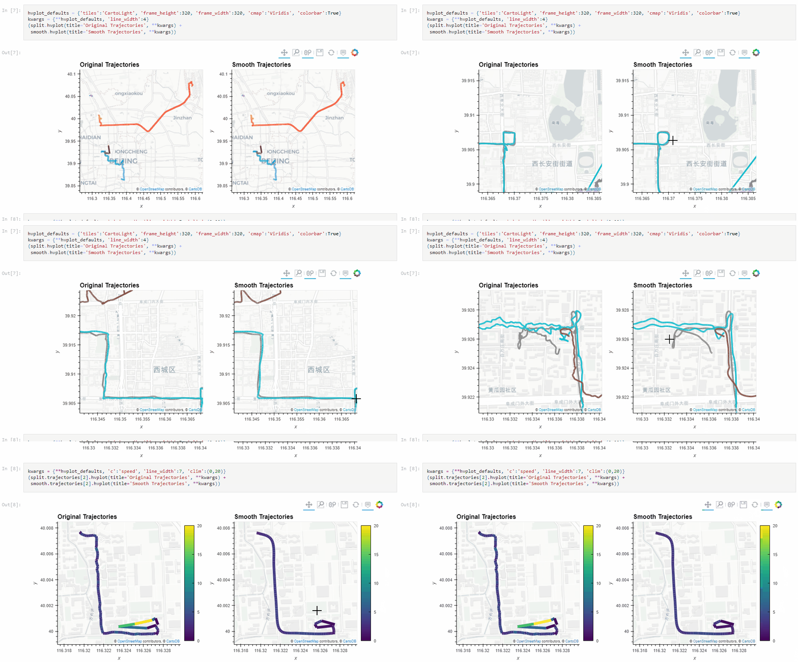
The Kalman filter in action on the Geolife sample: smoother, less jiggly trajectories.

Top-Down Time Ratio generalization aka trajectory compression in action: reduces the number of positions along the trajectory without altering the spatiotemporal properties, such as speed, too much.

These new algorithms were contributed by Lyudmil Vladimirov and George S. Theodoropoulos.

Behind the scenes, Ray Bell took care of moving testing from Travis to Github Actions, and together we worked through the steps to ensure that the source code is now properly linted using flake8 and black.

Being able to work with so many awesome contributors has made this release really special for me. It’s great to see the project attracting more developer interest.

As always, all tutorials are available from the movingpandas-examples repository and on MyBinder:

Snowy day map style now available on the QGIS hub

By underdark

2021-12-29

Cartography, QGIS

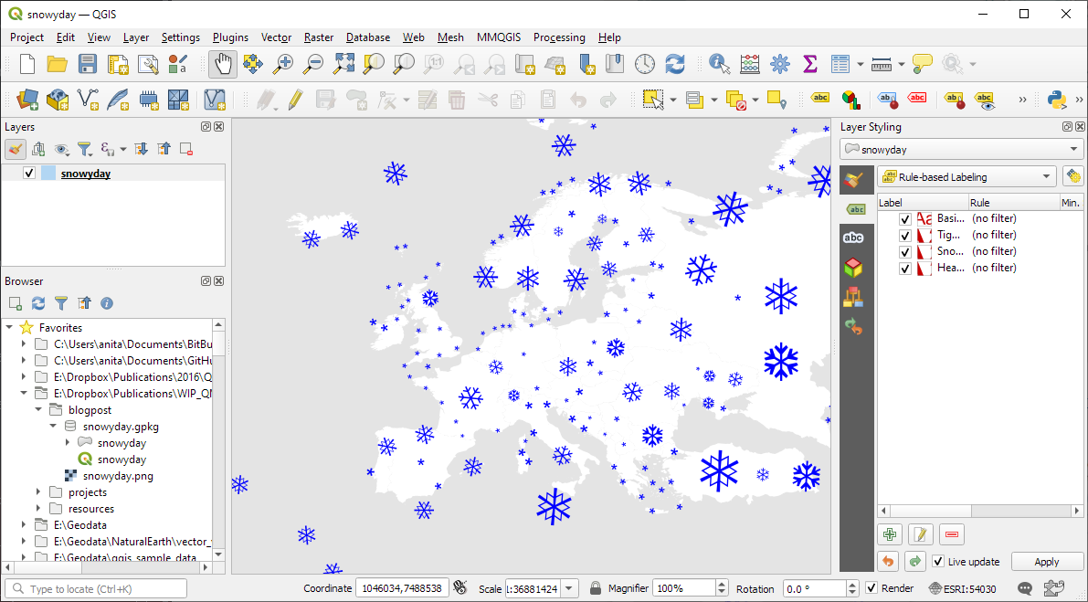
Today’s post is a follow-up and summary of my mapping efforts this December. It all started with a proof of concept that it is possible to create a nice looking snowfall effect using only labeling:

https://twitter.com/underdarkGIS/status/1470084114988650497

After a few more iterations, I even included the snowflake style in the first ever QGIS Map Design DLC: a free extra map recipe that shows how to create a map series of Antarctic expeditions. For more details (including project download links), check out my guest post on the Locate Press blog:

QGIS Map Design – Free Christmas DLC

If you want to just use the snowflake style in your own projects, the easiest way is to grab the “Snowy Day” project from the QGIS hub (while the GeoPackage is waiting for approval on the official site, you can get it from my Dropbox):

The project is self-contained within the downloaded GeoPackage. One of the most convenient ways to open projects from GeoPackages is through the browser panel:

From here, you can copy-paste the layer style to any other polygon layer.

To change the snowflake color, go to the project properties and edit the “flake_color” variable.

Happy new year!

New MovingPandas website

By underdark

2021-11-27

GIS

1 Comment

The last couple of days, I have been hacking away to improve the online presence of MovingPandas.

The new home page aims to be the central landing page that provides direct links to all important resources: from source code on Github, to documentation on ReadTheDocs, and – most importantly – all the tutorial and analysis example notebooks:

Additionally, all tutorial and analysis example notebooks now contain direct links to live versions on MyBinder, sources on Github and already executed pre-rendered HTML versions of the notebooks for quick browsing:

If you are using MovingPandas, I’d love to hear about it, particularly if you want to share one of your analysis examples with the community.

Open source for open spatial data science

By underdark

2021-11-12

GIS

1 Comment

Thanks to the FOSS4G2021 video team, all talks – including my keynote – are now available online.

I had the honor to be invited to give the closing keynote, talking about how open source can help open science, particularly data science:

I’m convinced that efforts towards more open data science are a worthwhile investment even if current scientific incentive structures are stacked against it.

Until incentive policies catch up, we all can help encourage more people to go the extra mile(s) by properly valuing their efforts, e.g. by celebrating and citing reproducible publications, open research datasets, and open scientific software.

Exploring ZAMG’s new open weather data

By underdark

2021-11-01

GIS, QGIS, spatio-temporal data

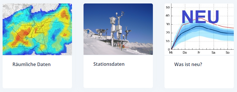
The Central Institution for Meteorology and Geodynamics (ZAMG) is Austrian’s meteorological and geophysical service. And as such, they have a large database of historical weather data which they have now made publicly available, as announced on 28th Oct 2021:

The new ZAMG Data Hub provides weather and station data, mainly in NetCDF and CSV formats:

I decided to grab a NetCDF sample from their analysis and nowcasting system INCA. I went with all available parameters for a period of one day (the data has a temporal resolution of one hour) and a bounding box around Vienna:

https://frontend.hub.zamg.ac.at/grid/d512d5b5-4e9f-4954-98b9-806acbf754f6/historical/form?anonymous=true

The loading screen of QGIS 3.22 shows the different NetCDF layers:

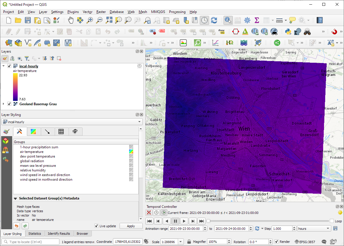
After adding the incal-hourly layer to QGIS, the layer styling panel provides access to the different weather parameters. We can switch between these parameters by clicking the gradient icon next to the parameter names. Here you can see the air temperature:

And because the NetCDF layer is time-aware, we can also use the QGIS Temporal Controller to step through the hourly measurements / create an animation:

Make sure to grab the latest version of QGIS to get access to all the functionality shown here.

MovingPandas v0.8 released!

By underdark

2021-11-01

MovingPandas

1 Comment

The latest v0.8 release is now available from conda-forge.

New features include:

More convenient creation of TrajectoryCollection objects from (Geo)DataFrames (#137)
Support for different geometry column names (#112)

Last week, I also had the pleasure to speak about MovingPandas at Carto’s Spatial Data Science Conference SDSC21:

As always, all tutorials are available from the movingpandas-examples repository and on MyBinder:

Movement data in GIS #37: “Understanding Movement Data” webinar

By underdark

2021-09-28

Movement data in GIS

Two weeks ago, I had the pleasure to speak at SystemX’s seminar series. The talk features a live demonstration of my protocol for exploring movement data, powered by Jupyter, Pandas, Holoviews, Datashader, GeoPandas, and MovingPandas. So if you haven’t read the paper yet, here’s the chance to watch the talk version:

This post is part of a series. Read more about movement data in GIS.

Exploring Vienna’s street-level Lidar “Kappazunder” data sample

By underdark

2021-09-25

QGIS

5 Comments

Kappazunder is the city of Vienna’s database created during their recent mobile mapping campaign. Using vehicle-mounted Lidar and cameras, they collected street-level Lidar and street view images.

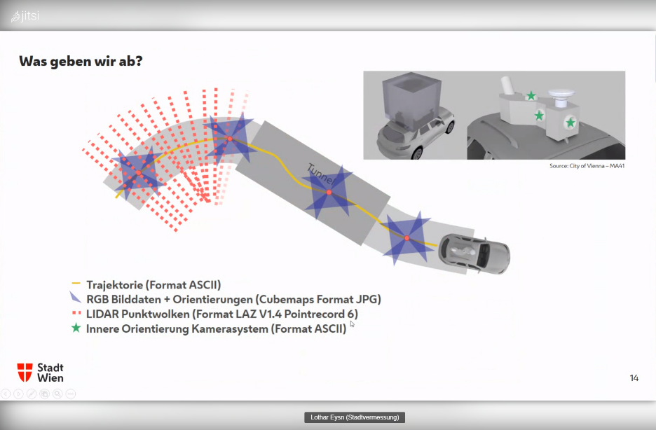
Slide from the official announcement on Thursday, 23rd Sept 2021. Full slide deck: https://www.slideshare.net/DigitalesWien/kappazunder-testdatensatz-2020-ogd-wien

Yesterday, they published a first sample dataset, containing one trajectory on data.gv.at. The download contains documentation, vector data (.shp), images (.jpg), and point clouds (.laz):

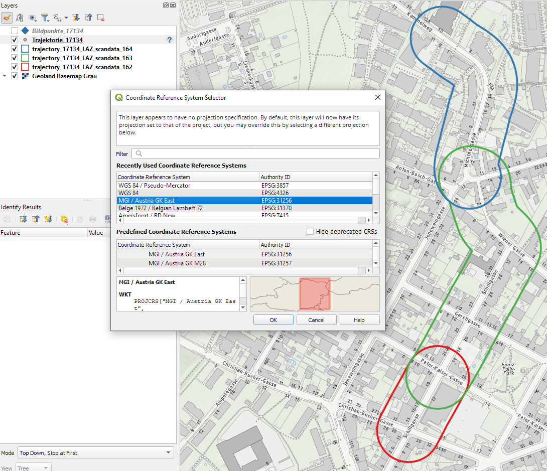
Trajectory

The shapefiles contain vehicle location updates, photo locations, and areas describing the extent of the point clouds. Since the shapefile lack .prj files, we need to manually specify the correct CRS (EPSG:31256 MGI / Austria GK East).

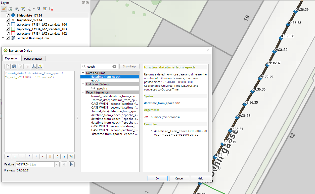
The vehicle location updates and photo locations contain timestamps as epoch. However, the format is a little special:

To display a human-readable timestamp, I therefore used the following label expression:

format_date( datetime_from_epoch( "epoch_s"*1000), 'HH:mm:ss')

Adding these labels also reveals that the whole trajectory is just 2 minutes long. This puts the download size of over 5GB into perspective. The whole dataset will be massive.

Lidar

The .laz files are between 100 and 200MB, each. There are four .laz files, even though the previously loaded point cloud extent areas only suggested three:

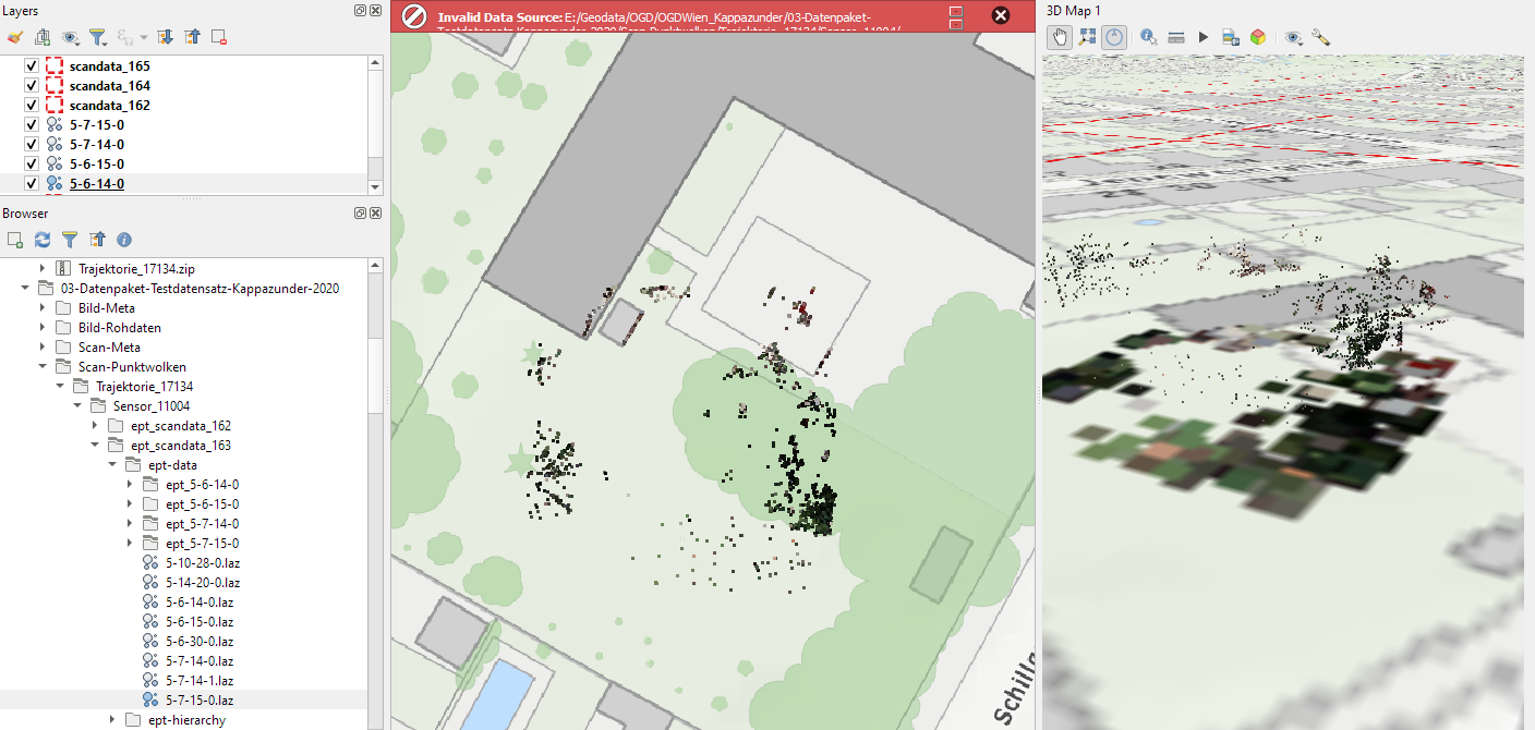
Loading the .laz files for the first time takes a while and there seem to be some issues – either on the user end (me) or in the files themselves. Trying to load content of the ept_ folders only results in very few points and multiple “invalid data source” errors:

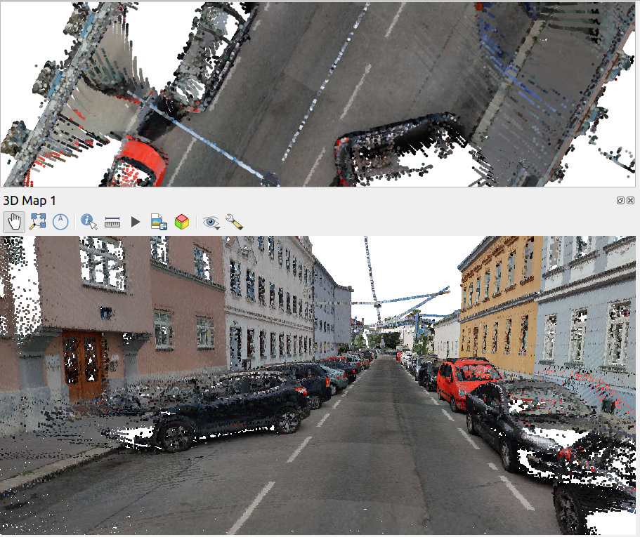
For the few point that are loaded, it looks like the height information is available:

Update on 2021-10-01: I’ve reported the data loss issue and Martin Dobias has provided a first work-around that makes it possible to view the data in QGIS: