Archive

GIS

Today’s post was motivated by a question over on gis.stackexchange, basically: How to draw a line with a gradient?

The issue we have to deal with is there is no gradient line style yet … But there are polygon gradient fills. So we can buffer the line and style the buffers. It’s a bit of an exercise in data-defined styling though:

Screenshot 2015-01-11 22.49.41

Before creating the buffer layer, we need to add the coordinates of the line start and end node to the line attributes. This is easy to do using the Field Calculator functions xat and yat, for example xat(0) for the x coordinate of the start node and yat(-1) for the y coordinate of the end node.

Screenshot 2015-01-11 22.41.37

Then we can buffer the lines and start styling the buffers. As mentioned, we’ll use the Gradient fill Symbol layer type.
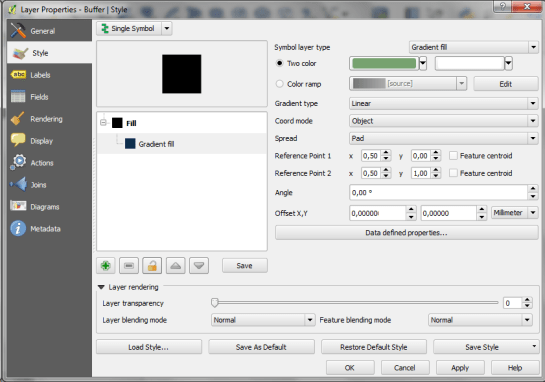
Screenshot 2015-01-11 22.49.54

The interesting part happens in the Data-defined properties. The start and end colors are computed from the measurement values from_m and to_m. Next, it’s important to use the feature coordinate mode because this will ensure that the coordinate system for the color gradient is based on the feature extent (with [0,0] in the upper left corner of the feature bbox).

Once that’s set up, we can compute the gradient start and end positions based on the line start and end node locations which we added to the attribute table in the beginning. If you’re wondering why Reference point 1 y is based on to_y (y coordinate of the line end point) rather than from_y, it’s due to the difference in coordinate origins in the geometry and the color gradient coordinate space: [0,0] is the lower left corner for the geometries but the upper left corner for the color gradient.
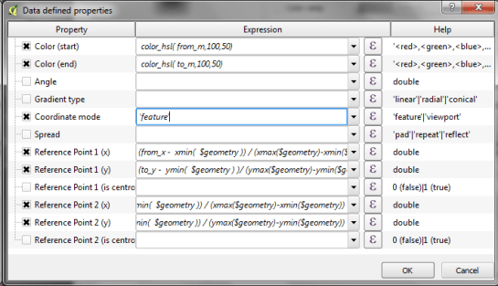
Screenshot 2015-01-11 22.42.35

As the title suggests, this is a really hackish solution for gradient line symbols. It will only provide reasonable results for straight – or close to straight – lines. But I’m very confident that we’ll have a real gradient line style in QGIS sooner or later.

Today’s post is a follow-up to a recent map experiment which I published in the QGIS Flickr group. It’s basically an inverted Stamen Toner style with an image in the map composition background instead of a solid color (similar to the approach described for vintage maps):

https://twitter.com/underdarkGIS/status/550340277257650176

That’s nice but with this approach we only get to enjoy the complete design in the print composer but not in the main window. So what other options do we have? – SVG fills to the rescue!

But first we need a suitable SVG with this nice pastel style. I used Gimp to create a seamless version of the pastel image and then embedded the image in an SVG using Inkscape:

LT_RemixedChalkPastel_snakk_seamless

In QGIS, this SVG can now be used in any SVG fill. It’s important to set the Texture width setting to a quite high value when working with SVGs containing big textures, otherwise the images will be rendered very small and the repeating patterns will be very obvious.

Screenshot 2015-01-04 17.49.11

Once the background is in place, we can add the line work and labels. The roads are white with black outlines for bridges which – together with the Lighten blending mode – produce the desired effect:

Screenshot 2015-01-04 17.37.33

Thank you for a great 2014! It’s been a pleasure to see the open source GIS community grow and experience what we can create together. It’s great to see the interest for open source GIS all over the world:

In total, this blog has been visitied from 216 countries. Most visitors came from The United States. Germany & France were not far behind.

In total, this blog has been visitied from 216 countries. Most visitors came from The United States. Germany & France were not far behind.

Since my first post in 2010, the development of this blog has exceeded all expectations I might have had by far. For 2014, the WordPress blog view counter shows a staggering 330,000 views or over 900 views per day.

In case you were wondering, the most popular posts of 2014 were:

  1. 3D Viz with QGIS & three.js
  2. A guide to GoogleMaps-like maps with OSM in QGIS
  3. A QGIS 2.2 preview
  4. Getting started writing QGIS 2.x plugins
  5. and Toner-lite styles for QGIS

Thank you, your feedback has been a continuous source of motivation. All the best for 2015!

It’s the end of December and time to recap 2014. Therefore, I decided to have a look at what this year has brought us. There were plenty of great posts for both casual and power users as well as developers. Here is my pick of the top 10 posts from the QGIS Planet blog aggregator.

  1. Tons of colour improvements! (Nyall Dawson)
  2. The QGIS Field calculator is dead. Long live the Field calculator bar (Nathan Woodrow)
  3. Why QGIS Class Names Start with Qgs (Gary Sherman)
  4. Atlas Previews (Nyall Dawson)
  5. QGIS atlas on non geometry tables (Nathan Woodrow)
  6. Gradient Fills (Nyall Dawson)
  7. What are all these QGIS file types? Why do I need them (Nathan Woodrow)
  8. Getting Started Writing QGIS Python Plugins (Peter Wells)
  9. QGIS Layer Tree API (Martin Dobias)
  10. Shapeburst fill styles (Nyall Dawson)

More great features and posts are sure to come next year. For example, Nyall is currently running a campaign on Kickstarter to add Live Layer Effects such as drop shadow effects to QGIS. Please support it if you can.

It’s my pleasure to announce that the updated and extended 2nd edition of Learning QGIS is available now.

I also want to take this opportunity to thank everyone who made the 1st edition such a great success!

This second edition has been updated to QGIS 2.6 and it features a completely new 6th chapter on Expanding QGIS with Python. It introduces the QGIS Python Console, shows how to create custom Processing tools, and provides a starting point for developing plugins.

Overall, the book has grown by 40 pages and the price of the print version has dropped by 3€ :-)

Happy QGISing!

2031OSos_mockupcover_normal_0

Correct turn restriction information is essential for the vehicle routing quality of any street network dataset – open or commercial. One of the challenges of this kind of information is that these restrictions are typically not directly visible on each map.

This post is inspired by a share on G+ which resurfaced in my notifications. In a post on the Mapbox blog, John Firebaugh presents the OSM iD editor which should make editing turn restrictions straight-forward: clicking on the source link turns the associated turn information visible. By clicking on the turn arrows, the user can easily toggle between allowed and forbidden.

iD, the web editor for OpenStreetMap, makes it even simpler to add turn restrictions to OpenStreetMap.

editing turn restrictions in iD, the web editor for OpenStreetMap. source: “Simple Editing for Turn Restrictions in OpenStreetMap” by John Firebaugh on June 06 2014

But the issue of identifying wrong turn restrictions remains. One approach to solving this issue is to compare restriction information in OSM with the information in a reference data set.

This is possible by comparing routes computed on OSM and the reference data using a method I presented at FOSS4G (video): a turn restriction basically is a forbidden combination of links. If we compute the route from the start link of the forbidden combination to the end link, we can check if the resulting route geometry violates the restriction or uses an appropriate detour:

read more about this method and results:

illustrative slide from my LBS2014 presentation on OSM vehicle routing quality – read more about this method and results for Vienna in our TGIS paper or the open pre-print version

It would be great to have an automated system comparing OSM and open government street network data to detect these differences. The quality of both data sets could benefit enormously by bundling their QA efforts. Unfortunately, the open government street network data sets I’m aware of don’t contain turn information.

The QGIS documentations team has released an updated version of the user guide:

qgisdocs26

I’d like to encourage everyone to have a look and explore the content, for example the great tips in the Actions menu section:

action_dialog

On my quest to create test data for spatial statistics, I’ve discovered income data for Austria per municipality on a news paper website:

Screenshot 2014-11-29 23.06.46

For further analysis, I decided to limit the area to Vienna and Lower Austria. Since the income data included GKZ “Gemeindekennzahl” IDs, it was possible to join them to municipalities extracted from OpenStreetMap using QuickOSM for QGIS. GRASS v.clean was used to clean the vector topology to the point where PySAL was able to compute spatial weights.

Using PySAL, I then computed income clusters: blue regions represent low clusters while red regions represent high clusters …

Municipality border data (c) OpenStreetMap and contributors Income data source: Statistik Austria via derStandard

Municipality border data (c) OpenStreetMap and contributors
Income data source: Statistik Austria via derStandard

The results show a statistically significant cluster of low income in the north west, in the area called Waldviertel, as well as a cluster of high income containing many of the municipalities surrounding Vienna, an area often referred to as the “Speckgürtel” (“bacon belt”).

Today, I’ve released TimeManager 1.2 which adds support for additional time formats: DD.MM.YYYY, DD/MM/YYYY, and DD-MM-YYYY (thanks to a pull request by vmora) as well as French translation (thanks to bbouteilles).

TimeManager now automatically detects formats such as DD.MM.YYYY

TimeManager now automatically detects formats such as DD.MM.YYYY

But there is more: the QGIS team has released a bugfix version 2.6.1 which you can already find in Ubuntu repos and the OSGeo4W installer. Go get it! And please support the bugfix release effort whenever you can.

As promised in my recent post “Experiments with Conway’s Game of Life”, I have been been looking into how to improve my first implementation. The new version which you can now find on Github is fully contained in one Python script which runs in the QGIS console. Additionally, the repository contains a CSV with the grid definition for a Gosper glider gun and the layer style QML.

Rather than creating a new Shapefile for each iteration like in the first implementation, this script uses memory layers to save the game status.

You can see it all in action in the following video:

(video available in HD)

Thanks a lot to Nathan Woodrow for the support in getting the animation running!

Sometimes there are still hick-ups causing steps to be skipped but overall it is running nicely now. Another approach would be to change the layer attributes rather than creating more and more layers but I like to be able to go through all the resulting layers after they have been computed.