Archive

QGIS

The Central Institution for Meteorology and Geodynamics (ZAMG) is Austrian’s meteorological and geophysical service. And as such, they have a large database of historical weather data which they have now made publicly available, as announced on 28th Oct 2021:

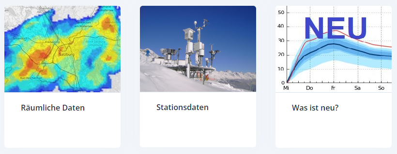
The new ZAMG Data Hub provides weather and station data, mainly in NetCDF and CSV formats:

I decided to grab a NetCDF sample from their analysis and nowcasting system INCA. I went with all available parameters for a period of one day (the data has a temporal resolution of one hour) and a bounding box around Vienna:

https://frontend.hub.zamg.ac.at/grid/d512d5b5-4e9f-4954-98b9-806acbf754f6/historical/form?anonymous=true

The loading screen of QGIS 3.22 shows the different NetCDF layers:

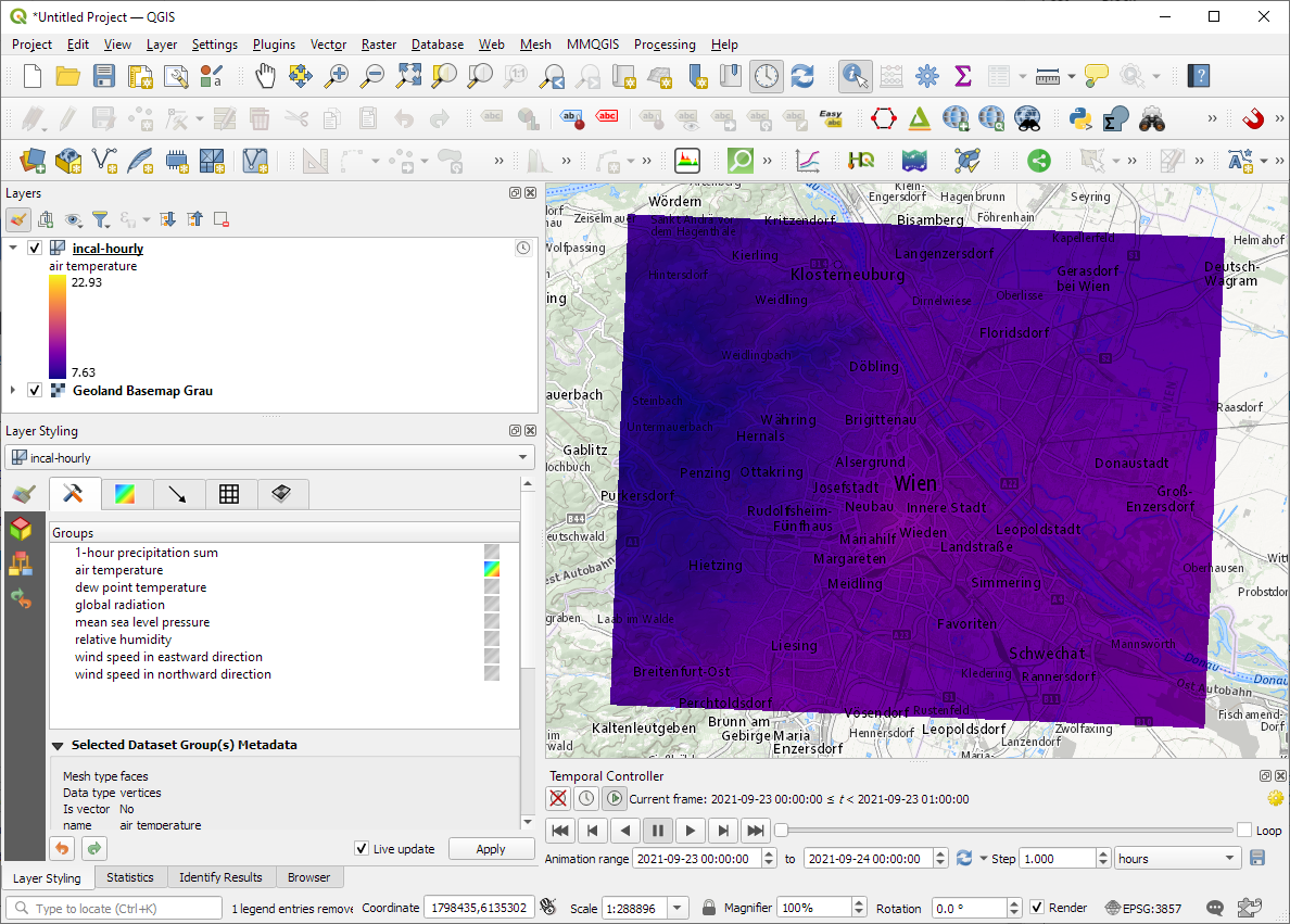
After adding the incal-hourly layer to QGIS, the layer styling panel provides access to the different weather parameters. We can switch between these parameters by clicking the gradient icon next to the parameter names. Here you can see the air temperature:

And because the NetCDF layer is time-aware, we can also use the QGIS Temporal Controller to step through the hourly measurements / create an animation:

Make sure to grab the latest version of QGIS to get access to all the functionality shown here.

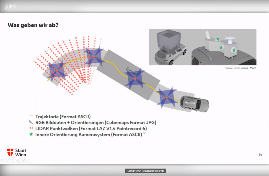
Kappazunder is the city of Vienna’s database created during their recent mobile mapping campaign. Using vehicle-mounted Lidar and cameras, they collected street-level Lidar and street view images.

Slide from the official announcement on Thursday, 23rd Sept 2021. Full slide deck: https://www.slideshare.net/DigitalesWien/kappazunder-testdatensatz-2020-ogd-wien

Yesterday, they published a first sample dataset, containing one trajectory on data.gv.at. The download contains documentation, vector data (.shp), images (.jpg), and point clouds (.laz):

Trajectory

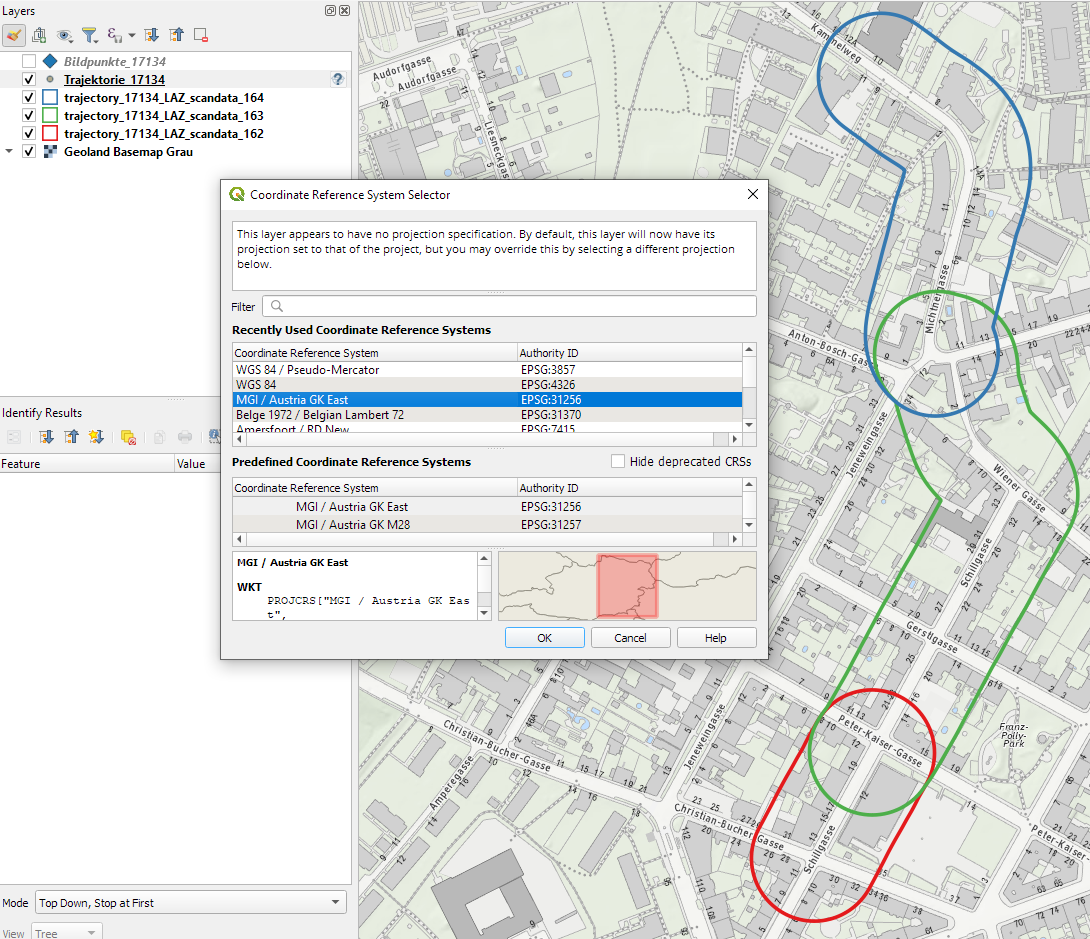
The shapefiles contain vehicle location updates, photo locations, and areas describing the extent of the point clouds. Since the shapefile lack .prj files, we need to manually specify the correct CRS (EPSG:31256 MGI / Austria GK East).

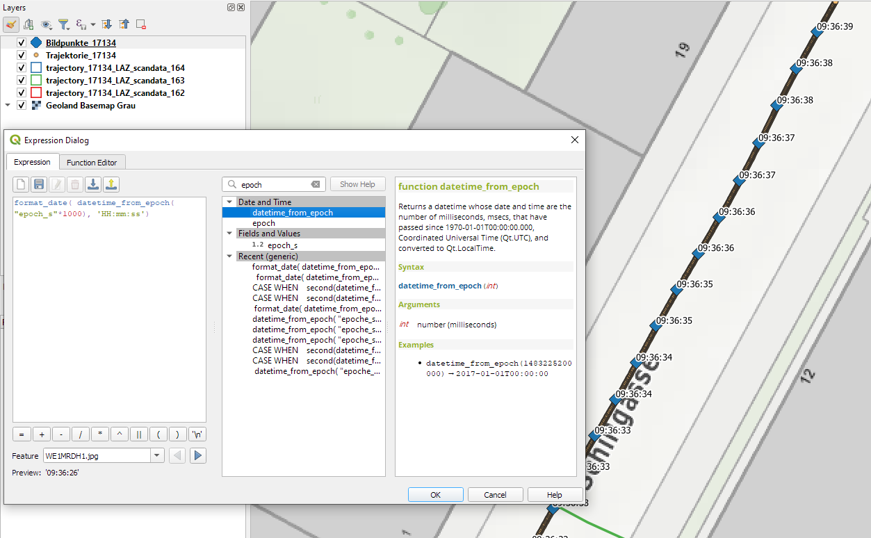
The vehicle location updates and photo locations contain timestamps as epoch. However, the format is a little special:

To display a human-readable timestamp, I therefore used the following label expression:

format_date( datetime_from_epoch( "epoch_s"*1000), 'HH:mm:ss')

Adding these labels also reveals that the whole trajectory is just 2 minutes long. This puts the download size of over 5GB into perspective. The whole dataset will be massive.

Lidar

The .laz files are between 100 and 200MB, each. There are four .laz files, even though the previously loaded point cloud extent areas only suggested three:

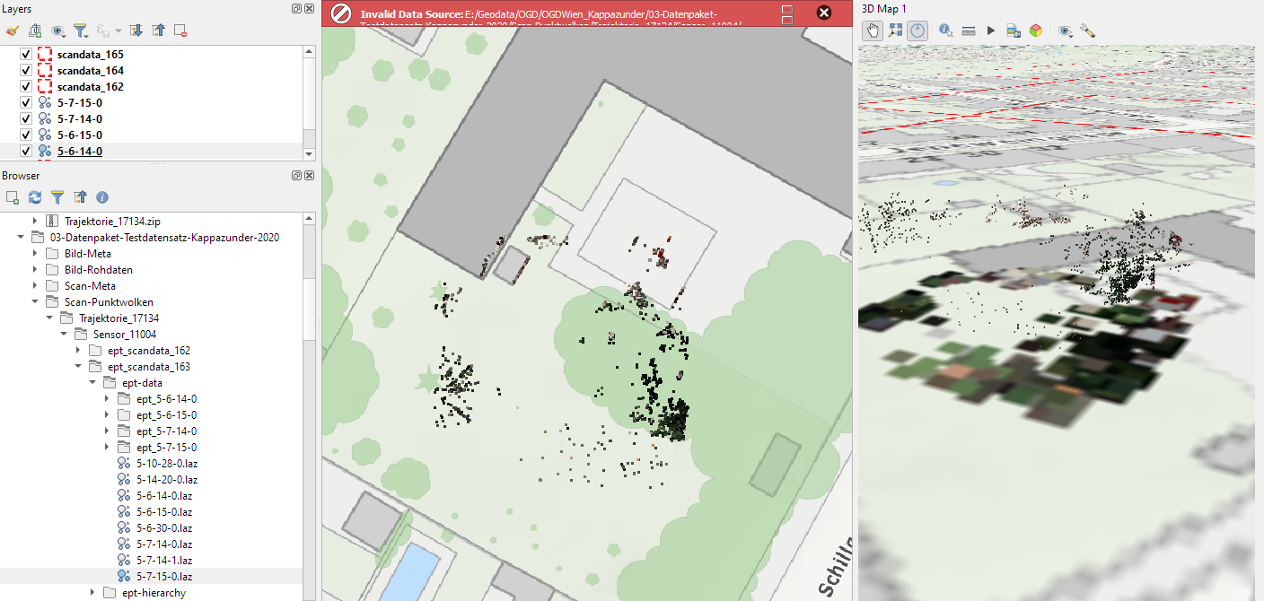
Loading the .laz files for the first time takes a while and there seem to be some issues – either on the user end (me) or in the files themselves. Trying to load content of the ept_ folders only results in very few points and multiple “invalid data source” errors:

For the few point that are loaded, it looks like the height information is available:

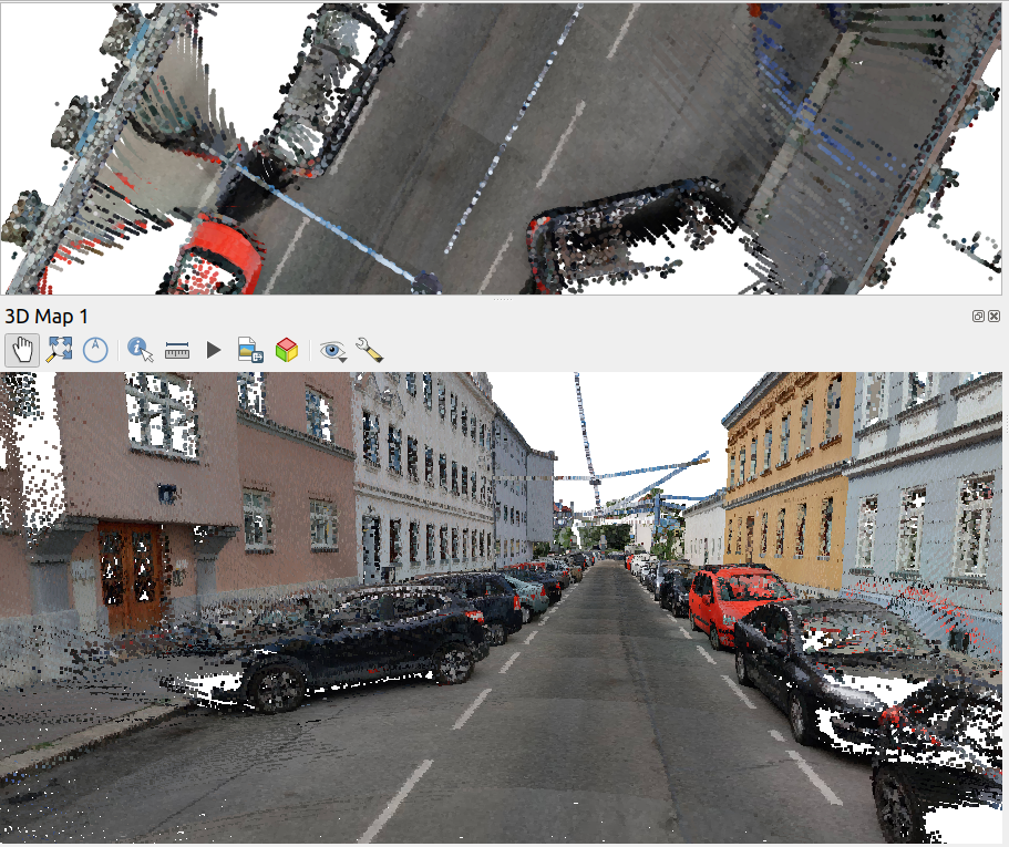
Update on 2021-10-01: I’ve reported the data loss issue and Martin Dobias has provided a first work-around that makes it possible to view the data in QGIS:

135284370-b07272bb-be8a-47ac-b050-d6024613c63b.png (911×765)

Images

The street view images are published as cubemaps. Here’s a sample of the side view:

One of the new features in QGIS 3.20 is the option to trim the start and end of simple line symbols. This allows for the line rendering to trim off the first and last sections of a line at a user configured distance, as shown in the visual changelog entry. 

This new feature makes it much easier to create decorative label callout (or leader) lines. If you know QGIS Map Design 2, the following map may look familiar – however – the following leader lines are even more intricate, making use of the new trimming capabilities:

To demonstrate some of the possibilities, I’ve created a set of four black and four white leader line styles:

You can download these symbols from the QGIS style sharing platform: https://plugins.qgis.org/styles/101/ to use them in your projects. Have fun mapping!

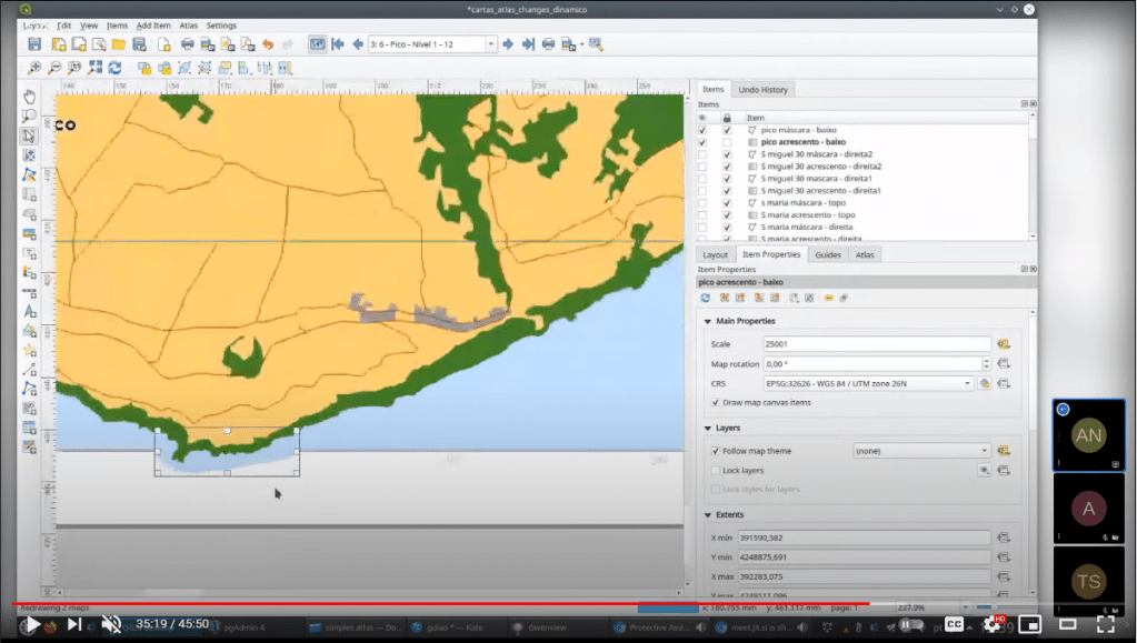
Today’s post is a video recommendation. In the following video, Alexandre Neto demonstrates an exciting array of tips, tricks, and hacks to create an automated Atlas map series of the Azores islands.

Highlights include:

1. A legend that includes automatically updating statistics

2. A way to support different page sizes

3. A solution for small areas overshooting the map border

You’ll find the video on the QGIS Youtube channel:

This video was recorded as part of the QGIS Open Day June edition. QGIS Open Days are organized monthly on the last Friday of the month. Anyone can take part and present their work for and with QGIS. For more details, see https://github.com/qgis/QGIS/wiki#qgis-open-day

If you are following QGIS topics on social media, you may have already seen this but if you don’t, I recommend having a look at Tim Sutton’s most recent adventures in building dashboards with QGIS:

https://twitter.com/timlinux/status/1333859727839784961

The dashboard is built using labeling and geometry generator functionality. This means that they work in the QGIS application map window as well as in layouts. As hinted at in the screenshot above, the dashboard can show information about whole layers as well as interactive selections.

Here’s a full walk-through Tim published yesterday:

You can follow the further development via Tim’s tweets or the dedicated Github issue (where you can even find an example QGIS dashboard project in a GeoPacakge for download).

Update July 2021: the style hub is now part of the official QGIS infrastructure at https://plugins.qgis.org/styles/


The 2016 post More icons & symbols for QGIS still regularly makes it to the top 10 list of posts by visitors. I wouldn’t attribute this popularity to the quality of this particular post, however. Instead, it’s a pretty clear sign that QGIS users are actively searching for more styling resources to add to their installations.

When it comes to styling resources, the person to follow right now is clearly Klas Karlsson who’s been keeping a steady stream of styling-related posts coming to Twitter:

Additionally, he’s the master-mind behind QGIS Hub, a – currently prototypical – platform for sharing styling resources and print layout templates:

If you are interested in sharing styling resources, head over there. Similarly, if you want to lend a hand developing QGIS Hub, get in touch!

QGIS Temporal Controller is a powerful successor of TimeManager. Temporal Controller is a new core feature of the current development version and will be shipped with the 3.14 release. This post demonstrates two key advantages of this new temporal support:

  1. Expression support for defining start and end timestamps
  2. Integration into the PyQGIS API

These features come in very handy in many use cases. For example, they make it much easier to create animations from folders full of GPS tracks since the files can now be loaded and configured automatically:

Script & Temporal Controller in action (click for full resolution)

All tracks start at the same location but at different times. (Kudos for Andrew Fletcher for recordings these tracks and sharing them with me!) To create an animation that shows all tracks start simultaneously, we need to synchronize them. This synchronization can be achieved on-the-fly by subtracting the start time from all track timestamps using an expression:

directory = "E:/Google Drive/QGIS_Course/05_TimeManager/Example_Dayrides/"

def load_and_configure(filename):
    path = os.path.join(directory, filename)
    uri = 'file:///' + path + "?type=csv&escape=&useHeader=No&detectTypes=yes"
    uri = uri + "&crs=EPSG:4326&xField=field_3&yField=field_2"
    vlayer = QgsVectorLayer(uri, filename, "delimitedtext")
    QgsProject.instance().addMapLayer(vlayer)

    mode = QgsVectorLayerTemporalProperties.ModeFeatureDateTimeStartAndEndFromExpressions
    expression = """to_datetime(field_1) -
    make_interval(seconds:=minimum(epoch(to_datetime("field_1")))/1000)
    """

    tprops = vlayer.temporalProperties()
    tprops.setStartExpression(expression)
    tprops.setEndExpression(expression) # optional
    tprops.setMode(mode)
    tprops.setIsActive(True)

for filename in os.listdir(directory):
    if filename.endswith(".csv"):
        load_and_configure(filename)

The above script loads all CSV files from the given directory (field_1 is the timestamp, field_2 is y, and field_3 is x), enables sets the start and end expression as well as the corresponding temporal control mode and finally activates temporal rendering. The resulting config can be verified in the layer properties dialog:

To adapt this script to other datasets, it’s sufficient to change the file directory and revisit the layer uri definition as well as the field names referenced in the expression.


This post is part of a series. Read more about movement data in GIS.

TimeManager turns 10 this year. The code base has made the transition from QGIS 1.x to 2.x and now 3.x and it would be wrong to say that it doesn’t show ;-)

Now, it looks like the days of TimeManager are numbered. Four days ago, Nyall Dawson has added native temporal support for vector layers to QGIS. This is part of a larger effort of adding time support for rasters, meshes, and now also vectors.

The new Temporal Controller panel looks similar to TimeManager. Layers are configured through the new Temporal tab in Layer Properties. The temporal dimension can be used in expressions to create fancy time-dependent styles:

temporal1

TimeManager Geolife demo converted to Temporal Controller (click for full resolution)

Obviously, this feature is brand new and will require polishing. Known issues listed by Nyall include limitations of supported time fields (only fields with datetime type are supported right now, strings cannot be used) and worse performance than TimeManager since features are filtered in QGIS rather than in the backend.

If you want to give the new Temporal Controller a try, you need to install the current development version, e.g. qgis-dev in OSGeo4W.


Update from May 16:

Many of the limitations above have already been addressed.

Last night, Nyall has recorded a one hour tutorial on this new feature, enjoy:

Mapping spatial decision patterns, such as election results, is always a hot topic. That’s why we decided to include a recipe for election maps in our QGIS Map Design books. What’s new is that this recipe is now available as a free video tutorial recorded by Oliver Burdekin:

This video is just one of many recently published video tutorials that have been created by QGIS community members.

For example, Hans van der Kwast and Kurt Menke have recorded a 7-part series on QGIS for Hydrological Applications:

and Klas Karlsson’s Youtube channel is also always worth a follow:

For the Pythonically inclined among you, there is also a new version of Python in QGIS on the Automating GIS-processes channel:


In the past, network analysis capabilities in QGIS were rather limited or not straight-forward to use. This has changed! In QGIS 3.x, we now have a wide range of network analysis tools, both for use case where you want to use your own network data, as well as use cases where you don’t have access to appropriate data or just prefer to use an existing service.

This blog post aims to provide an overview of the options:

  1. Based on local network data
    1. Default QGIS Processing network analysis tools
    2. QNEAT3 plugin
  2. Based on web services
    1. Hqgis plugin (HERE)
    2. ORS Tools plugin (openrouteservice.org)
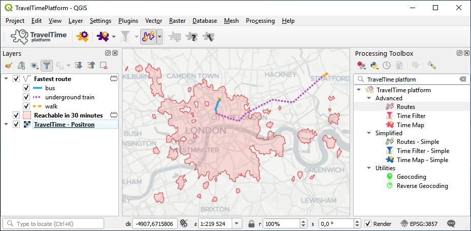
    3. TravelTime platform plugin (TravelTime platform)

All five options provide Processing toolbox integration but not at the same level.

If you are a regular reader of this blog, you’re probably also aware of the pgRoutingLayer plugin. However, I’m not including it in this list due to its dependency on PostGIS and its pgRouting extension.

Processing network analysis tools

The default Processing network analysis tools are provided out of the box. They provide functionality to compute least cost paths and service areas (distance or time) based on your own network data. Inputs can be individual points or layers of points:

The service area tools return reachable edges and / or nodes rather than a service area polygon:

QNEAT3 plugin

The QNEAT3 (short for Qgis Network Analysis Toolbox 3) Plugin aims to provide sophisticated QGIS Processing-Toolbox algorithms in the field of network analysis. QNEAT3 is integrated in the QGIS3 Processing Framework. It offers algorithms that range from simple shortest path solving to more complex tasks like Iso-Area (aka service areas, accessibility polygons) and OD-Matrix (Origin-Destination-Matrix) computation.

QNEAT3 is an alternative for use case where you want to use your own network data.

For more details see the QNEAT3 documentation at: https://root676.github.io/index.html

Hqgis plugin

Access the HERE API from inside QGIS using your own HERE-API key. Currently supports Geocoding, Routing, POI-search and isochrone analysis.

Hqgis currently does not expose all its functionality to the Processing toolbox:

Instead, the full set of functionality is provided through the plugin GUI:

This plugin requires a HERE API key.

ORS Tools plugin

ORS Tools provides access to most of the functions of openrouteservice.org, based on OpenStreetMap. The tool set includes routing, isochrones and matrix calculations, either interactive in the map canvas or from point files within the processing framework. Extensive attributes are set for output files, incl. duration, length and start/end locations.

ORS Tools is based on OSM data. However, using this plugin still requires an openrouteservice.org API key.

TravelTime platform plugin

This plugin adds a toolbar and processing algorithms allowing to query the TravelTime platform API directly from QGIS. The TravelTime platform API allows to obtain polygons based on actual travel time using several transport modes rather, allowing for much more accurate results than simple distance calculations.

The TravelTime platform plugin requires a TravelTime platform API key.

For more details see: https://blog.traveltimeplatform.com/isochrone-qgis-plugin-traveltime