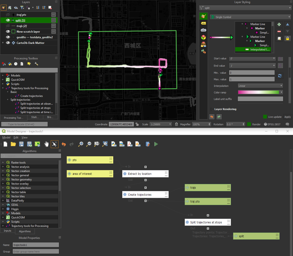
I’m continuously testing the algorithms integrated so far to see if they work as GIS users would expect and can to ensure that they can be integrated in Processing model seamlessly.
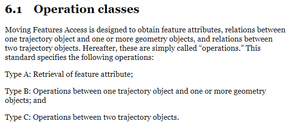
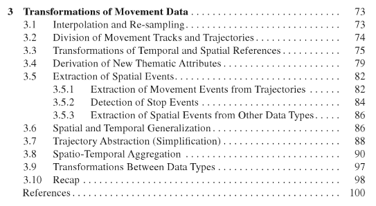
Because naming things is tricky, I’m currently struggling with how to best group the toolbox algorithms into meaningful categories. I looked into the categories mentioned in OGC Moving Features Access but honestly found them kind of lacking:
… but I’m not convinced yet. So take the above listed three categories with a grain of salt. Those may change before the release. (Any inputs / feedback / recommendation welcome!)
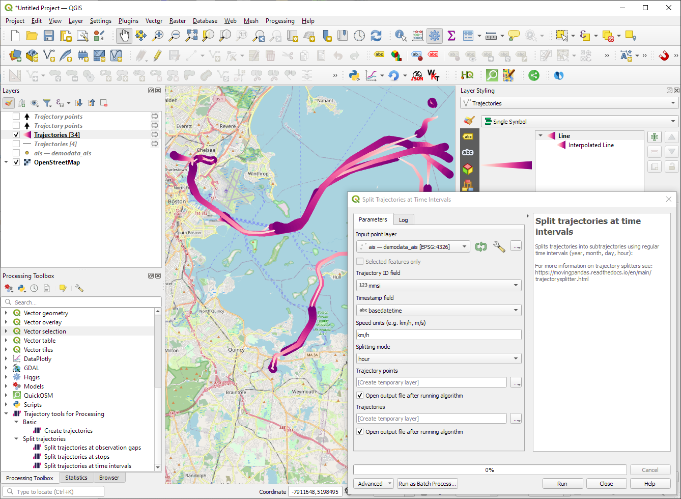
Let me close this quick status update with a screencast showcasing stop detection in AIS data, featuring the recently added trajectory styling using interpolated lines:
Trajectools development started back in 2018 but has been on hold since 2020 when I realized that it would be necessary to first develop a solid trajectory analysis library. With the MovingPandas library in place, I’ve now started to reboot Trajectools.
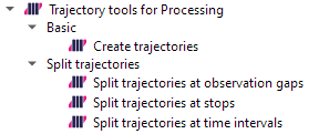
Trajectools v2 builds on MovingPandas and exposes its trajectory analysis algorithms in the QGIS Processing Toolbox. So far, I have integrated the basic steps of
Building trajectories including speed and direction information from timestamped points and
Splitting trajectories at observation gaps, stops, or regular time intervals.
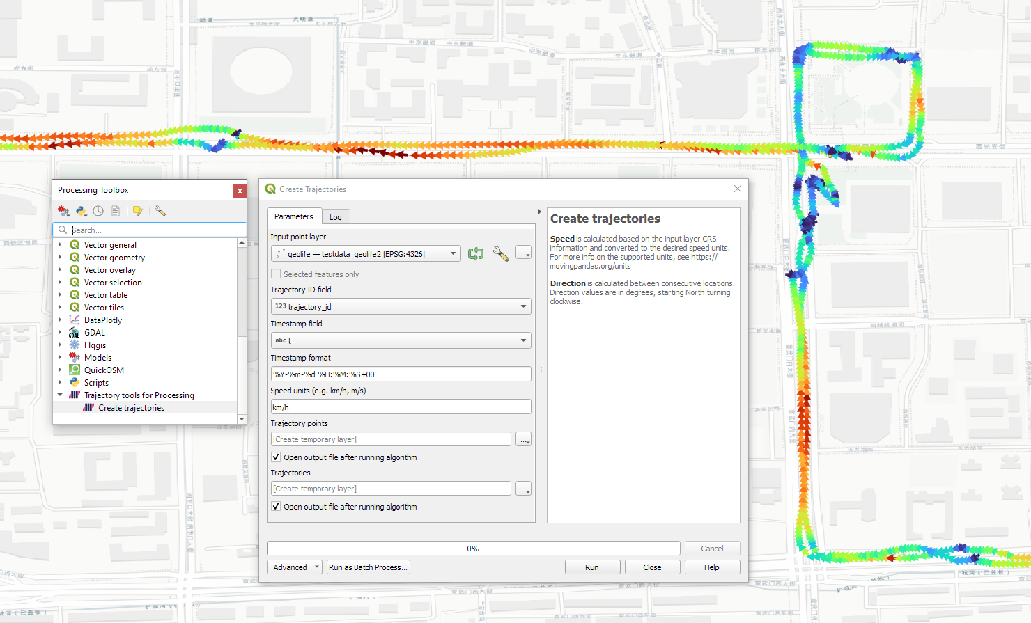
The algorithms create two output layers:
Trajectory points with speed and direction information that are styled using arrow markers
Trajectories as LineStringMs which makes it straightforward to count the number of trajectories and to visualize where one trajectory ends and another starts.
So far, the default style for the trajectory points is hard-coded to apply the Turbo color ramp on the speed column with values from 0 to 50 (since I’m simply loading a ready-made QML). By default, the speed is calculated as km/h but that can be customized:
I don’t have a solution yet to automatically create a style for the trajectory lines layer. Ideally, the style should be a categorized renderer that assigns random colors based on the trajectory id column. But in this case, it’s not enough to just load a QML.
In the meantime, I might instead include an Interpolated Line style. What do you think?
Of course, the goal is to make Trajectools interoperable with as many existing QGIS Processing Toolbox algorithms as possible to enable efficient Mobility Data Science workflows.
The easiest way to set up QGIS with MovingPandas Python environment is to install both from conda. You can find the instructions together with the latest Trajectools development version at: https://github.com/movingpandas/qgis-processing-trajectory
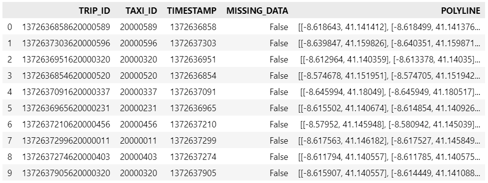
Kaggle’s “Taxi Trajectory Data from ECML/PKDD 15: Taxi Trip Time Prediction (II) Competition” is one of the most used mobility / vehicle trajectory datasets in computer science. However, in contrast to other similar datasets, Kaggle’s taxi trajectories are provided in a format that is not readily usable in MovingPandas since the spatiotemporal information is provided as:
TIMESTAMP: (integer) Unix Timestamp (in seconds). It identifies the trip’s start;
POLYLINE: (String): It contains a list of GPS coordinates (i.e. WGS84 format) mapped as a string. The beginning and the end of the string are identified with brackets (i.e. [ and ], respectively). Each pair of coordinates is also identified by the same brackets as [LONGITUDE, LATITUDE]. This list contains one pair of coordinates for each 15 seconds of trip. The last list item corresponds to the trip’s destination while the first one represents its start;
Therefore, we need to create a DataFrame with one point + timestamp per row before we can use MovingPandas to create Trajectories and analyze them.
But first things first. Let’s download the dataset:
import datetime
import pandas as pd
import geopandas as gpd
import movingpandas as mpd
import opendatasets as od
from os.path import exists
from shapely.geometry import Point

input_file_path = 'taxi-trajectory/train.csv'

def get_porto_taxi_from_kaggle():
    if not exists(input_file_path):
        od.download("https://www.kaggle.com/datasets/crailtap/taxi-trajectory")

get_porto_taxi_from_kaggle()
df = pd.read_csv(input_file_path, nrows=10, usecols=['TRIP_ID', 'TAXI_ID', 'TIMESTAMP', 'MISSING_DATA', 'POLYLINE'])
df.POLYLINE = df.POLYLINE.apply(eval)  # string to list
df
And now for the remodelling:
def unixtime_to_datetime(unix_time):
    return datetime.datetime.fromtimestamp(unix_time)

def compute_datetime(row):
    unix_time = row['TIMESTAMP']
    offset = row['running_number'] * datetime.timedelta(seconds=15)
    return unixtime_to_datetime(unix_time) + offset

def create_point(xy):
    try:
        return Point(xy)
    except TypeError:  # when there are nan values in the input data
        return None

new_df = df.explode('POLYLINE')
new_df['geometry'] = new_df['POLYLINE'].apply(create_point)
new_df['running_number'] = new_df.groupby('TRIP_ID').cumcount()
new_df['datetime'] = new_df.apply(compute_datetime, axis=1)
new_df.drop(columns=['POLYLINE', 'TIMESTAMP', 'running_number'], inplace=True)
new_df
And that’s it. Now we can create the trajectories:
That’s it. Now our MovingPandas.TrajectoryCollection is ready for further analysis.
By the way, the plot above illustrates a new feature in the recent MovingPandas 0.16 release which, among other features, introduced plots with arrow markers that show the movement direction. Other new features include a completely new custom distance, speed, and acceleration unit support. This means that, for example, instead of always getting speed in meters per second, you can now specify your desired output units, including km/h, mph, or nm/h (knots).
These releases are a huge step forward towards making MovingPandas easier to install with fewer mandatory dependencies. All interactive plotting libraries are now optional. So if you are using MovingPandas for trajectory data processing in the background and don’t need the interactive visualization features, the number of necessary libraries is now much lower. This (and the fact that GeoPandas is now shipped with OSGeo4W) will also make it easier to use MovingPandas in QGIS plugins.
We have further improved our repo setup by adding an action that automatically creates and publishes packages from releases, heavily inspired by the work of the GeoPandas team.
Last but not least, we’ve created a Twitter account for the project. (And might soon add a Mastodon account as well.)
As always, all tutorials are available from the movingpandas-examples repository and on MyBinder:
If you have questions about using MovingPandas or just want to discuss new ideas, you’re welcome to join our discussion forum.
New functions to add a timedelta column and get the trajectory sampling interval #233
As always, all tutorials are available from the movingpandas-examples repository and on MyBinder:
The new distance measures are covered in tutorial #11:
Computing distances between trajectories, as illustrated in tutorial #11Computing distances between a trajectory and other geometry objects, as illustrated in tutorial #11
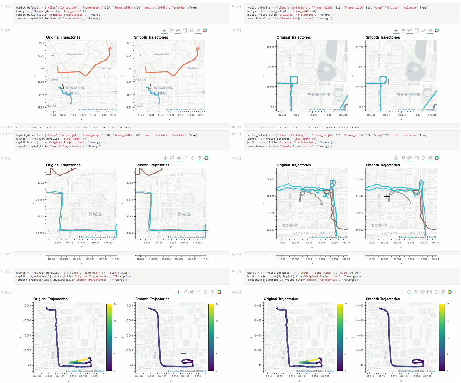
But don’t miss the great features covered by the other notebooks, such as outlier cleaning and smoothing:
Trajectory cleaning and smoothing, as illustrated in tutorial #10
If you have questions about using MovingPandas or just want to discuss new ideas, you’re welcome to join our discussion forum.
Speed and direction column names can now be customized
If you have questions about using MovingPandas or just want to discuss new ideas, you’re welcome to join our recently opened discussion forum.
As always, all tutorials are available from the movingpandas-examples repository and on MyBinder:
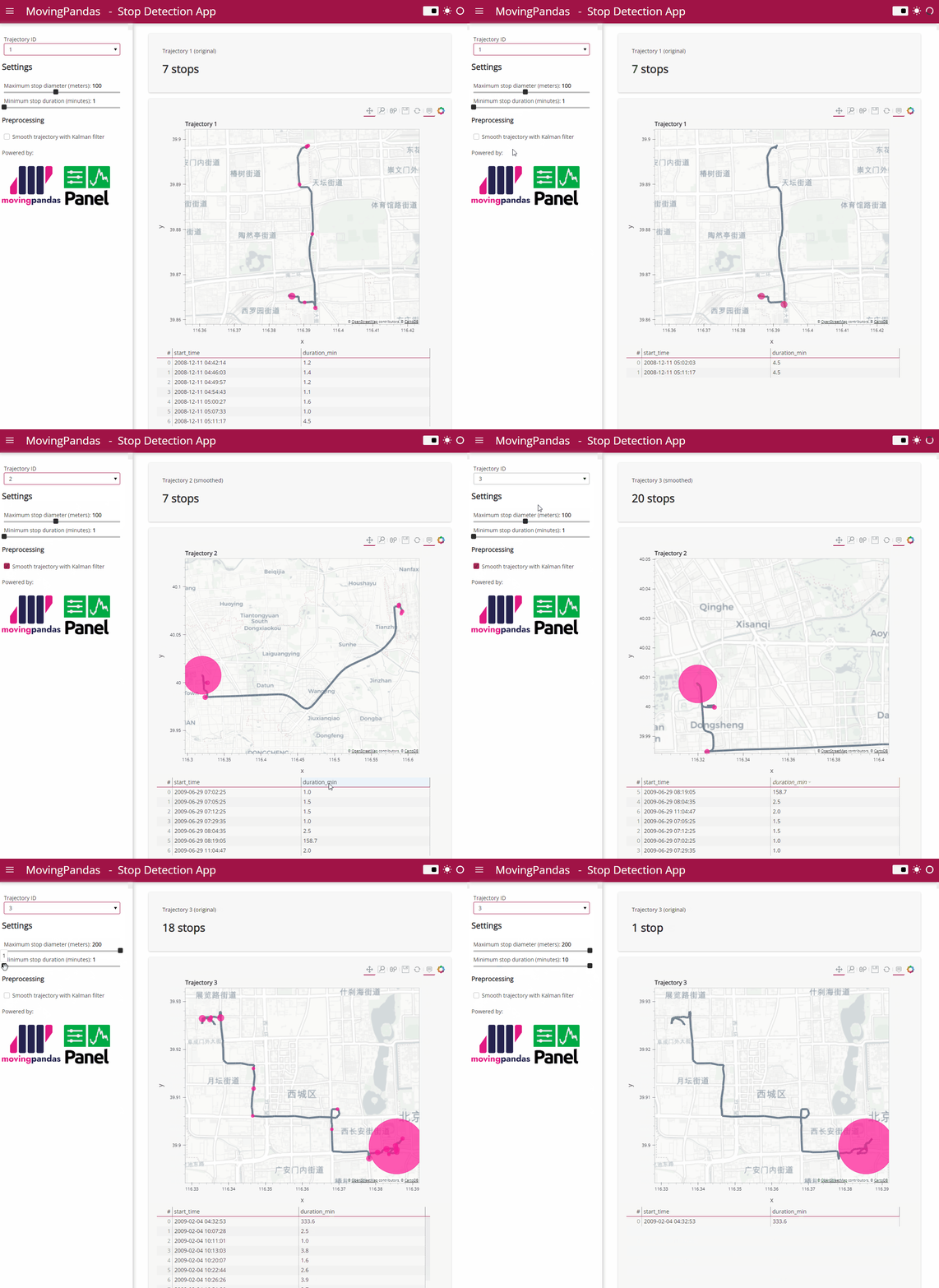
Besides others examples, the movingpandas-examples repo contains the following tech demo: an interactive app built with Panel that demonstrates different MovingPandas stop detection parameters
To start the app, open the stopdetection-app.ipynb notebook and press the green Panel button in the Jupyter Lab toolbar:
The Kalman filter in action on the Geolife sample: smoother, less jiggly trajectories.Top-Down Time Ratio generalization aka trajectory compression in action: reduces the number of positions along the trajectory without altering the spatiotemporal properties, such as speed, too much.
Behind the scenes, Ray Bell took care of moving testing from Travis to Github Actions, and together we worked through the steps to ensure that the source code is now properly linted using flake8 and black.
Being able to work with so many awesome contributors has made this release really special for me. It’s great to see the project attracting more developer interest.
As always, all tutorials are available from the movingpandas-examples repository and on MyBinder: