Today’s post is a follow-up of Movement data in GIS #3: visualizing massive trajectory datasets. In that post, I summarized a concept for trajectory generalization. Now, I have published the scripts and sample data in my QGIS-Processing-tools repository on Github.

To add the trajectory generalization scripts to your Processing toolbox, you can use the Add scripts from files tool:

It is worth noting, that Add scripts from files fails to correctly import potential help files for the scripts but that’s not an issue this time around, since I haven’t gotten around to actually write help files yet.

The scripts are used in the following order:

Extract characteristic trajectory points
Group points in space
Compute flows between cells from trajectories

The sample project contains input data, as well as output layers of the individual tools. The only required input is a layer of trajectories, where trajectories have to be LINESTRINGM (note the M!) features:

Trajectory sample based on data provided by the GeoLife project

In Extract characteristic trajectory points, distance parameters are specified in meters, stop duration in seconds, and angles in degrees. The characteristic points contain start and end locations, as well as turns and stop locations:

The characteristic points are then clustered. In this tool, the distance has to be specified in layer units, which are degrees in case of the sample data.

Finally, we can compute flows between cells defined by these clusters:

Flow lines scaled by flow strength and cell centers scaled by counts

If you use these tools on your own data, I’d be happy so see what you come up with!

This post is part of a series. Read more about movement data in GIS.

Movement data in GIS #8: edge bundling for flow maps

By underdark

2017-10-08

Movement data in GIS, QGIS, Visualization

24 Comments

If you follow this blog, you’ll probably remember that I published a QGIS style for flow maps a while ago. The example showed domestic migration between the nine Austrian states, a rather small dataset. Even so, it required some manual tweaking to make the flow map readable. Even with only 72 edges, the map quickly gets messy:

Raw migration flows between Austrian states, line width scaled by flow strength

One popular approach in the data viz community to deal with this problem is edge bundling. The idea is to reduce visual clutter by generate bundles of similar edges.

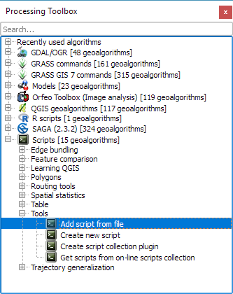
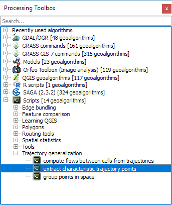
Surprisingly, edge bundling is not available in desktop GIS. Existing implementations in the visual analytics field often run on GPUs because edge bundling is computationally expensive. Nonetheless, we have set out to implement force-directed edge bundling for the QGIS Processing toolbox [0]. The resulting scripts are available on Github.

The main procedure consists of two tools: bundle edges and summarize. Bundle edges takes the raw straight lines, and incrementally adds intermediate nodes (called control points) and shifts them according to computed spring and electrostatic forces. If the input are 72 lines, the output again are 72 lines but each line geometry has been bent so that similar lines overlap and form a bundle.

After this edge bundling step, most common implementations compute a line heatmap, that is, for each map pixel, determine the number of lines passing through the pixel. But QGIS does not support line heatmaps and this approach also has issues distinguishing lines that run in opposite directions. We have therefore implemented a summarize tool that computes the local strength of the generated bundles.

Continuing our previous example, if the input are 72 lines, summarize breaks each line into its individual segments and determines the number of segments from other lines that are part of the same bundle. If a weight field is specified, each line is not just counted once but according to its weight value. The resulting bundle strength can be used to create a line layer style with data-defined line width:

Bundled migration flows

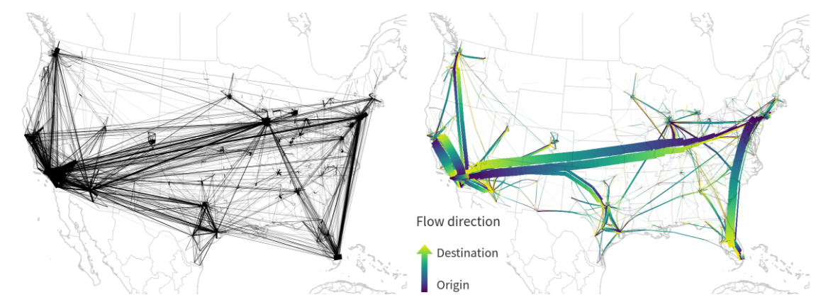
To avoid overlaps of flows in opposing directions, we define a line offset. Finally, summarize also adds a sequence number to the line segments. This sequence number is used to assign a line color on the gradient that indicates flow direction.

I already mentioned that edge bundling is computationally expensive. One reason is that we need to perform pairwise comparison of edges to determine if they are similar and should be bundled. This comparison results in a compatibility matrix and depending on the defined compatibility threshold, different bundles can be generated.

The following U.S. dataset contains around 4000 lines and bundling it takes a considerable amount of time.

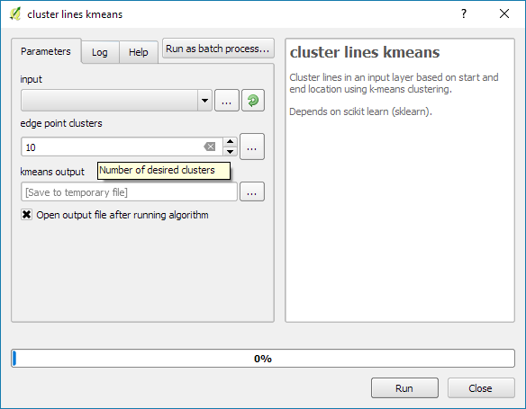
One approach to speed up computations is to first use a quick clustering algorithm and then perform edge bundling on each cluster individually. If done correctly, clustering significantly reduces the size of each compatibility matrix.

In this example, we divided the edges into six clusters before bundling them. If you compare this result to the visualization at the top of this post (which did not use clustering), you’ll see some differences here and there but, overall, the results are quite similar:

Looking at these examples, you’ll probably spot a couple of issues. There are many additional ideas for potential improvements from existing literature which we have not implemented yet. If you are interested in improving these tools, please go ahead! The code and more examples are available on Github.

For more details, leave your email in a comment below and I’ll gladly send you the pre-print of our paper.

[0] Graser, A., Schmidt, J., Roth, F., & Brändle, N. (2017 online) Untangling Origin-Destination Flows in Geographic Information Systems. Information Visualization – Special Issue on Visual Movement Analytics.

This post is part of a series. Read more about movement data in GIS.

Movement data in GIS #4: variations over time

By underdark

2016-11-20

Movement data in GIS, spatio-temporal data, Visualization

In the previous post, I presented an approach to generalize big trajectory datasets by extracting flows between cells of a data-driven irregular grid. This generalization provides a much better overview of the flow and directionality than a simple plot of the original raw trajectory data can. The paper introducing this method also contains more advanced visualizations that show cell statistics, such as the overall count of trajectories or the generalization quality. Another bit of information that is often of interest when exploring movement data, is the time of the movement. For example, at LBS2016 last week, M. Jahnke presented an application that allows users to explore the number of taxi pickups and dropoffs at certain locations:

Jahnke, M., Ding, L., Karja, K., & Wang, S. (2017). Identifying Origin/Destination Hotspots in Floating Car Data for Visual Analysis of Traveling Behavior. In Progress in Location-Based Services 2016 (pp. 253-269). Springer International Publishing.

By adopting this approach for the generalized flow maps, we can, for example, explore which parts of the research area are busy at which time of the day. Here I have divided the day into four quarters: night from 0 to 6 (light blue), morning from 6 to 12 (orange), afternoon from 12 to 18 (red), and evening from 18 to 24 (dark blue).

Aggregated trajectories with time-of-day markers at flow network nodes (data credits: GeoLife project, map tiles: Carto, map data: OSM)

The resulting visualization shows that overall, there is less movement during the night hours from midnight to 6 in the morning (light blue quarter). Sounds reasonable!

One implementation detail worth considering is which timestamp should be used for counting the number of movements. Should it be the time of the first trajectory point entering a cell, or the time when the trajectory leaves the cell, or some average value? In the current implementation, I have opted for the entry time. This means that if the tracked person spends a long time within a cell (e.g. at the work location) the trip home only adds to the evening trip count of the neighboring cell along the trajectory.

Since the time information stored in a PostGIS LinestringM feature’s m-value does not contain any time zone information, we also have to pay attention to handle any necessary offsets. For example, the GeoLife documentation states that all timestamps are provided in GMT while Beijing is in the GMT+8 time zone. This offset has to be accounted for in the analysis script, otherwise the counts per time of day will be all over the place.

Using the same approach, we could also investigate other variations, e.g. over different days of the week, seasonal variations, or the development over multiple years.

This post is part of a series. Read more about movement data in GIS.

Visualizing direction-dependent values

By underdark

2014-07-21

GIS, QGIS

7 Comments

When mapping flows or other values which relate to a certain direction, styling these layers gets interesting. I faced the same challenge when mapping direction-dependent error values. Neighboring cell pairs were connected by two lines, one in each direction, with an associated error value. This is what I came up with:

Each line is drawn with an offset to the right. The size of the offset depends on the width of the line which in turn depends on the size of the error. You can see the data-defined style properties here:

To indicate the direction, I added a marker line with one > marker at the center. This marker line also got assigned the same offset to match the colored line bellow. I’m quite happy with how these turned out and would love to hear about your approaches to this issue.

These figures are part of a recent publication with my AIT colleagues: A. Graser, J. Asamer, M. Dragaschnig: “How to Reduce Range Anxiety? The Impact of Digital Elevation Model Quality on Energy Estimates for Electric Vehicles” (2014).

Data-defined properties in QGIS 2.0

By underdark

2013-06-04

QGIS

8 Comments

In QGIS 2.0, the old “size scale” field has been replaced by data-defined properties which enable us to control many more properties than jut size and rotation. One of the often requested features – for example – is the possibility for data-defined colors:

Today’s example map visualizes a dataset of known meteorite landings published on http://visualizing.org/datasets/meteorite-landings. I didn’t clean the data, so there is quite a bunch of meteorites at 0/0.

To create the map, I used QGIS 2.0 feature blending mode “multiply” as well as data-defined size based on meteorite mass:

Background oceans and graticule by NaturalEarthData.

Mapping the Night

By underdark

2012-03-09

QGIS, Visualization

8 Comments

Most maps of night time lights show the land masses lit brightly by city lights. But the oceans are not as dark as these maps suggest. NOAA/NGDC datasets available through edenextdata.com show very bright spots in the North Sea:

Night time lights trace the coast but illuminate the sea too.

The dataset description mentions that the sensors pick up moonlit clouds, lights from human settlements, fires, gas flares, heavily lit fishing boats, lightning and the aurora. So might these spots be fishing boats?

Update: As many comments have pointed out, bright spots in the seas show the locations of oil drilling rigs.

Visualizing Global Connections

By underdark

2011-08-20

GIS, PostGIS, QGIS, Visualization

19 Comments

Today, I’ve been experimenting with data from OpenFlights.org. They offer airport, airline and route data for download. The first idea that came to mind was to connect airports on a shared route by lines. This kind of visualization just looks much nicer if the connections are curved instead of simple straight lines.

Luckily, that’s pretty easy to do using PostGIS. After loading airport positions and route data, we can create the connection lines like this (based on [postgis-users] Great circle as a linestring):

UPDATE experimental.airroutes
SET the_geom = 
(SELECT ST_Transform(ST_Segmentize(ST_MakeLine(
       ST_Transform(a.the_geom, 953027),
       ST_Transform(b.the_geom, 953027)
     ), 100000 ), 4326 ) 
 FROM experimental.airports a, experimental.airports b
 WHERE a.id = airroutes.source_id  
   AND b.id = airroutes.dest_id
);

The CRS used in the query is not available in PostGIS by default. You can add it like this (source: spatialreference.org):

INSERT into spatial_ref_sys (srid, auth_name, auth_srid, proj4text, srtext) values ( 953027, 'esri', 53027, '+proj=eqdc +lat_0=0 +lon_0=0 +lat_1=60 +lat_2=60 +x_0=0 +y_0=0 +a=6371000 +b=6371000 +units=m +no_defs ', 'PROJCS["Sphere_Equidistant_Conic",GEOGCS["GCS_Sphere",DATUM["Not_specified_based_on_Authalic_Sphere",SPHEROID["Sphere",6371000,0]],PRIMEM["Greenwich",0],UNIT["Degree",0.017453292519943295]],PROJECTION["Equidistant_Conic"],PARAMETER["False_Easting",0],PARAMETER["False_Northing",0],PARAMETER["Central_Meridian",0],PARAMETER["Standard_Parallel_1",60],PARAMETER["Standard_Parallel_2",60],PARAMETER["Latitude_Of_Origin",0],UNIT["Meter",1],AUTHORITY["EPSG","53027"]]');

This is an example visualization (done in QGIS) showing only flight routes starting from Vienna International Airport:

Flight routes from Vienna International

Connections crossing the date line are currently more problematic. Lines would have to be split, otherwise this is what you’ll get:

Date line trouble

Visualizing Traffic Velocities in a Network

By underdark

2011-03-25

Network, Visualization

“The Morphing City” by Pedro M Cruz is a visualization of deviations of traffic velocities in the city of Lisbon:

The Morphing City from Pedro M Cruz on Vimeo.

Very inspiring!

VisualEyes – A Visualization Tool for Spatio-temporal Data

By underdark

2010-11-23

GIS, spatio-temporal data, Visualization

VisualEyes is an online tool developed at the University of Virginia. It allows you to combine images, maps, charts, video and data into interactive dynamic visualizations.

The examples offer multiple map layers, charts and of course a time slider to navigate through time.