Detecting close encounters using MobilityDB 1.0

It’s been a while since we last talked about MobilityDB in 2019 and 2020. Since then, the project has come a long way. It joined OSGeo as a community project and formed a first PSC, including the project founders Mahmoud Sakr and Esteban Zimányi as well as Vicky Vergara (of pgRouting fame) and yours truly.

This post is a quick teaser tutorial from zero to computing closest points of approach (CPAs) between trajectories using MobilityDB.

Setting up MobilityDB with Docker

The easiest way to get started with MobilityDB is to use the ready-made Docker container provided by the project. I’m using Docker and WSL (Windows Subsystem Linux on Windows 10) here. Installing WLS/Docker is out of scope of this post. Please refer to the official documentation for your operating system.

Once Docker is ready, we can pull the official container and fire it up:

docker pull mobilitydb/mobilitydb
docker volume create mobilitydb_data
docker run --name "mobilitydb" -d -p 25432:5432 -v mobilitydb_data:/var/lib/postgresql mobilitydb/mobilitydb
psql -h localhost -p 25432 -d mobilitydb -U docker

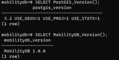
Currently, the container provides PostGIS 3.2 and MobilityDB 1.0:

Loading movement data into MobilityDB

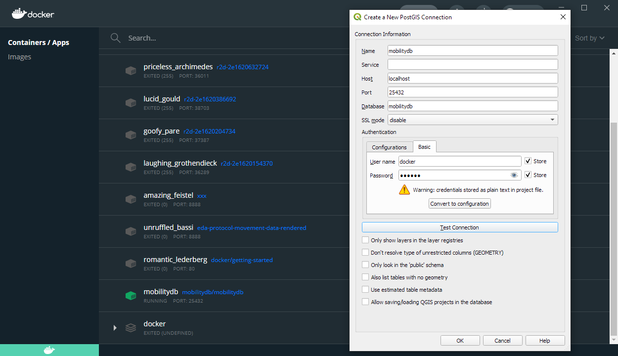
Once the container is running, we can already connect to it from QGIS. This is my preferred way to load data into MobilityDB because we can simply drag-and-drop any timestamped point layer into the database:

For this post, I’m using an AIS data sample in the region of Gothenburg, Sweden.

After loading this data into a new table called ais, it is necessary to remove duplicate and convert timestamps:

CREATE TABLE AISInputFiltered AS
SELECT DISTINCT ON("MMSI","Timestamp") *
FROM ais;

ALTER TABLE AISInputFiltered ADD COLUMN t timestamp;
UPDATE AISInputFiltered SET t = "Timestamp"::timestamp;

Afterwards, we can create the MobilityDB trajectories:

CREATE TABLE Ships AS
SELECT "MMSI" mmsi,
tgeompoint_seq(array_agg(tgeompoint_inst(Geom, t) ORDER BY t)) AS Trip,
tfloat_seq(array_agg(tfloat_inst("SOG", t) ORDER BY t) FILTER (WHERE "SOG" IS NOT NULL) ) AS SOG,
tfloat_seq(array_agg(tfloat_inst("COG", t) ORDER BY t) FILTER (WHERE "COG" IS NOT NULL) ) AS COG
FROM AISInputFiltered
GROUP BY "MMSI";

ALTER TABLE Ships ADD COLUMN Traj geometry;
UPDATE Ships SET Traj = trajectory(Trip);

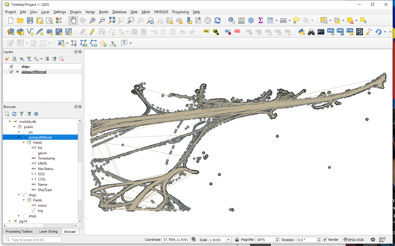
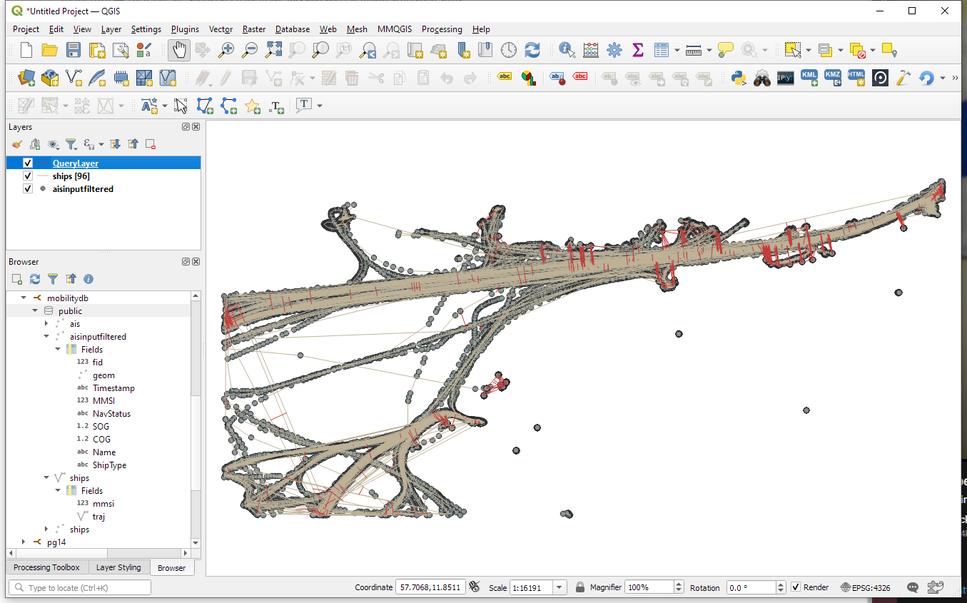
Once this is done, we can load the resulting Ships layer and the trajectories will be loaded as lines:

Computing closest points of approach

To compute the closest point of approach between two moving objects, MobilityDB provides a shortestLine function. To be correct, this function computes the line connecting the nearest approach point between the two tgeompoint_seq. In addition, we can use the time-weighted average function twavg to compute representative average movement speeds and eliminate stationary or very slowly moving objects:

SELECT S1.MMSI mmsi1, S2.MMSI mmsi2, 
       shortestLine(S1.trip, S2.trip) Approach,
       ST_Length(shortestLine(S1.trip, S2.trip)) distance
FROM Ships S1, Ships S2
WHERE S1.MMSI > S2.MMSI AND
twavg(S1.SOG) > 1 AND twavg(S2.SOG) > 1 AND
dwithin(S1.trip, S2.trip, 0.003)

In the QGIS Browser panel, we can right-click the MobilityDB connection to bring up an SQL input using Execute SQL:

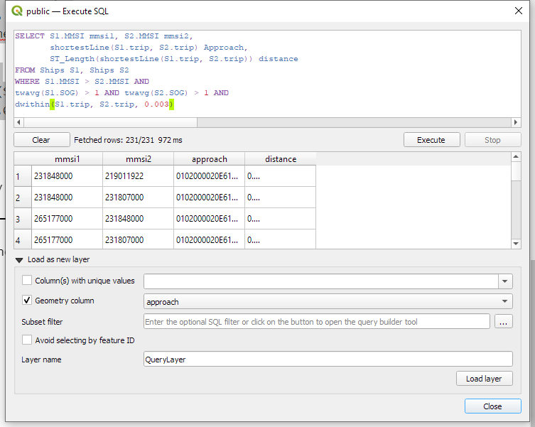
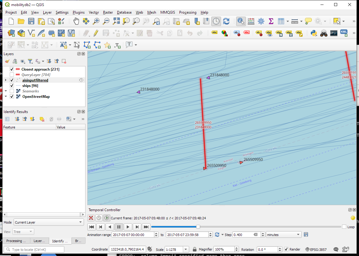
The resulting query layer shows where moving objects get close to each other:

To better see what’s going on, we’ll look at individual CPAs:

Having a closer look with the Temporal Controller

Since our filtered AIS layer has proper timestamps, we can animate it using the Temporal Controller. This enables us to replay the movement and see what was going on in a certain time frame.

I let the animation run and stopped it once I spotted a close encounter. Looking at the AIS points and the shortest line, we can see that MobilityDB computed the CPAs along the trajectories:

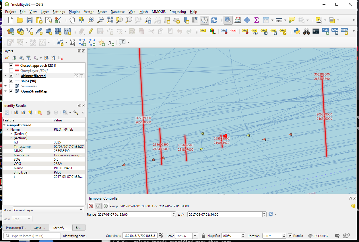
A more targeted way to investigate a specific CPA is to use the Temporal Controllers’ fixed temporal range mode to jump to a specific time frame. This is helpful if we already know the time frame we are interested in. For the CPA use case, this means that we can look up the timestamp of a nearby AIS position and set up the Temporal Controller accordingly: