Archive

Tag Archives: PostGIS

Recently there has been some buzz on Twitter about a new moving object database (MOD) called MobilityDB that builds on PostgreSQL and PostGIS (Zimányi et al. 2019). The MobilityDB Github repo has been published in February 2019 but according to the following presentation at PgConf.Russia 2019 it has been under development for a few years:

Of course, moving object databases have been around for quite a while. The two most commonly cited MODs are HermesDB (Pelekis et al. 2008) which comes as an extension for either PostgreSQL or Oracle and is developed at the University of Piraeus and SECONDO (de Almeida et al. 2006) which is a stand-alone database system developed at the Fernuniversität Hagen. However, both MODs remain at the research prototype level and have not achieved broad adoption.

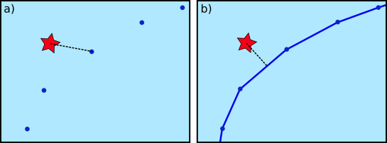
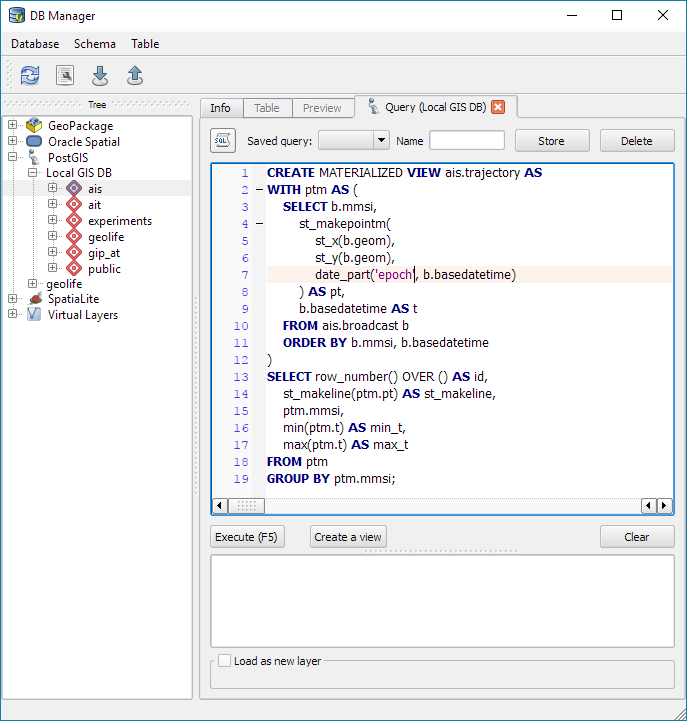
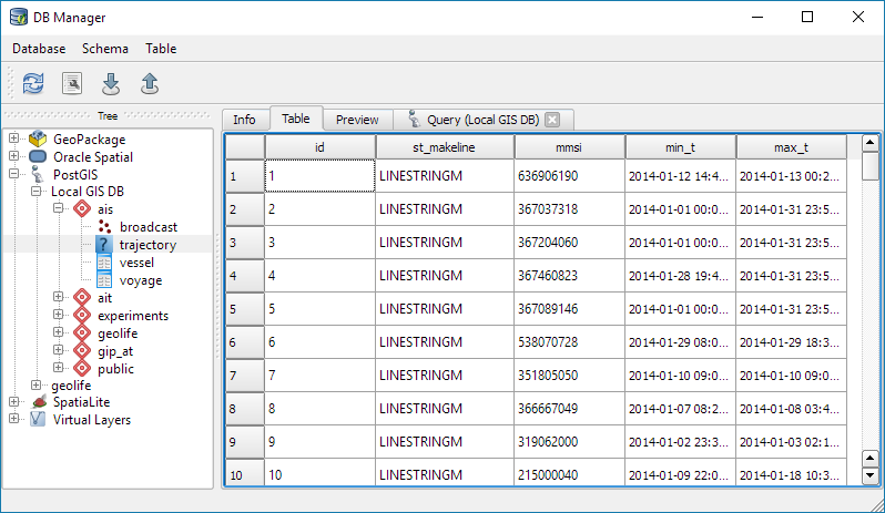
It will be interesting to see if MobilityDB will be able to achieve the goal they have set in the title of Zimányi et al. (2019) to become “a mainstream moving object database system”. It’s promising that they are building on PostGIS and using its mature spatial analysis functionality instead of reinventing the wheel. They also discuss why they decided that PostGIS trajectories (which I’ve written about in previous posts) are not the way to go:

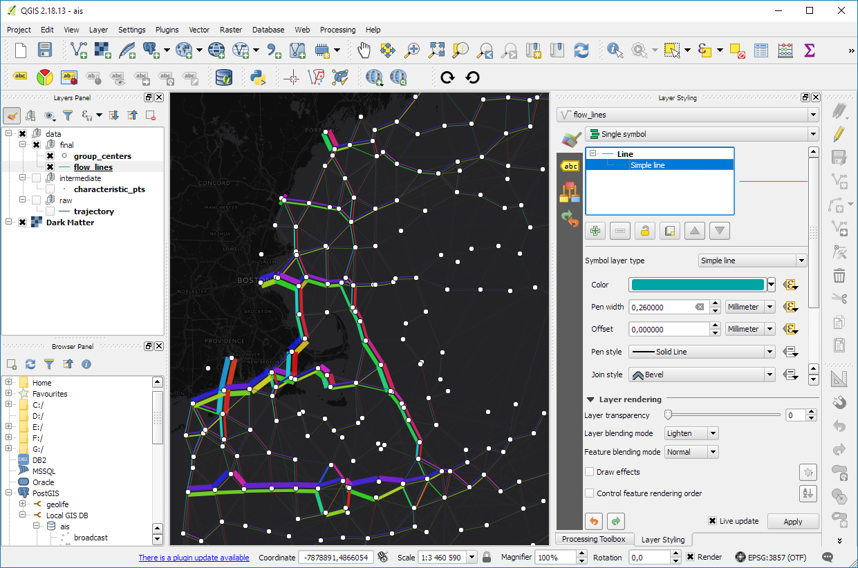
However, the presentation does not go into detail whether there are any straightforward solutions to visualizing data stored in MobilityDB.

According to the Github readme, MobilityDB runs on Linux and needs PostGIS 2.5. They also provide an online demo as well as a Docker container with MobilityDB and all its dependencies. If you give it a try, I would love to hear about your experiences.

References

  • de Almeida, V. T., Guting, R. H., & Behr, T. (2006). Querying moving objects in secondo. In 7th International Conference on Mobile Data Management (MDM’06) (pp. 47-47). IEEE.
  • Pelekis, N., Frentzos, E., Giatrakos, N., & Theodoridis, Y. (2008). HERMES: aggregative LBS via a trajectory DB engine. In Proceedings of the 2008 ACM SIGMOD international conference on Management of data (pp. 1255-1258). ACM.
  • Zimányi, E., Sakr, M., Lesuisse, A., & Bakli, M. (2019). MobilityDB: A Mainstream Moving Object Database System. In Proceedings of the 16th International Symposium on Spatial and Temporal Databases (pp. 206-209). ACM.

This post is part of a series. Read more about movement data in GIS.

Today’s post continues where “Why you should be using PostGIS trajectories” leaves off. It’s the result of a collaboration with Eva Westermeier. I had the pleasure to supervise her internship at AIT last year and also co-supervised her Master’s thesis [0] on the topic of enriching trajectories with information about their geographic context.

Context-aware analysis of movement data is crucial for different domains and applications, from transport to ecology. While there is a wealth of data, efficient and user-friendly contextual trajectory analysis is still hampered by a lack of appropriate conceptual approaches and practical methods. (Westermeier, 2018)

Part of the work was focused on evaluating different approaches to adding context information from vector datasets to trajectories in PostGIS. For example, adding land cover context to animal movement data or adding information on anchoring and harbor areas to vessel movement data.

Classic point-based model vs. line-based model

The obvious approach is to intersect the trajectory points with context data. This is the classic point data model of contextual trajectories. It’s straightforward to add context information in the point-based model but it also generates large numbers of repeating annotations. In contrast, the line data model using, for example, PostGIS trajectories (LinestringM) is more compact since trajectories can be split into segments at context borders. This creates one annotation per segment and the individual segments are convenient to analyze (as described in part #12).

Spatio-temporal interpolation as provided by the line data model offers additional advantages for the analysis of annotated segments. Contextual segments start and end at the intersection of the trajectory linestring with context polygon borders. This means that there are no gaps like in the point-based model. Consequently, while the point-based model systematically underestimates segment length and duration, the line-based approach offers more meaningful segment length and duration measurements.

Schematic illustration of a subset of an annotated trajectory in two context classes, a) systematic underestimation of length or duration in the point data model, b) full length or duration between context polygon borders in the line data model (source: Westermeier (2018))

Another issue of the point data model is that brief context changes may be missed or represented by just one point location. This makes it impossible to compute the length or duration of the respective context segment. (Of course, depending on the application, it can be desirable to ignore brief context changes and make the annotation process robust towards irrelevant changes.)

Schematic illustration of context annotation for brief context changes, a) and b)
two variants for the point data model, c) gapless annotation in the line data model (source: Westermeier (2018) based on Buchin et al. (2014))

Beyond annotations, context can also be considered directly in an analysis, for example, when computing distances between trajectories and contextual point objects. In this case, the point-based approach systematically overestimates the distances.

Schematic illustration of distance measurement from a trajectory to an external
object, a) point data model, b) line data model (source: Westermeier (2018))

The above examples show that there are some good reasons to dump the classic point-based model. However, the line-based model is not without its own issues.

Issues

Computing the context annotations for trajectory segments is tricky. The main issue is that ST_Intersection drops the M values. This effectively destroys our trajectories! There are ways to deal with this issue – and the corresponding SQL queries are published in the thesis (p. 38-40) – but it’s a real bummer. Basically, ST_Intersection only provides geometric output. Therefore, we need to reconstruct the temporal information in order to create usable trajectory segments.

Finally, while the line-based model is well suited to add context from other vector data, it is less useful for context data from continuous rasters but that was beyond the scope of this work.

Conclusion

After the promising results of my initial investigations into PostGIS trajectories, I was optimistic that context annotations would be a straightforward add-on. The line-based approach has multiple advantages when it comes to analyzing contextual segments. Unfortunately, generating these contextual segments is much less convenient and also slower than I had hoped. Originally, I had planned to turn this work into a plugin for the Processing toolbox but the results of this work motivated me to look into other solutions. You’ve already seen some of the outcomes in part #20 “Trajectools v1 released!”.

References

[0] Westermeier, E.M. (2018). Contextual Trajectory Modeling and Analysis. Master Thesis, Interfaculty Department of Geoinformatics, University of Salzburg.


This post is part of a series. Read more about movement data in GIS.

Do you sometimes start writing an SQL query and around at line 50 you get the feeling that it might be getting out of hand? If so, it might be useful to start breaking it down into smaller chunks and wrap those up into custom functions. Never done that? Don’t despair! There’s an excellent PL/pgSQL tutorial on postgresqltutorial.com to get you started.

To get an idea of the basic structure of a PL/pgSQL function and to proof that PostGIS datatypes work just fine in this context, here’s a basic function that takes a trajectory geometry and outputs its duration, i.e. the difference between its last and first timestamp:

CREATE OR REPLACE FUNCTION AG_Duration(traj geometry) 
RETURNS numeric LANGUAGE 'plpgsql'
AS $BODY$ 
BEGIN
RETURN ST_M(ST_EndPoint(traj))-ST_M(ST_StartPoint(traj));
END; $BODY$;

My end goal for this exercise was to implement a function that takes a trajectory and outputs the stops along this trajectory. Commonly, a stop is defined as a long stay within an area with a small radius. This leads us to the following definition:

CREATE OR REPLACE FUNCTION AG_DetectStops(
   traj geometry, 
   max_size numeric, 
   min_duration numeric)
RETURNS TABLE(sequence integer, geom geometry) 
-- implementation follows here!

Note how this function uses RETURNS TABLE to enable it to return all the stops that it finds. To add a line to the output table, we need to assign values to the sequence and geom variables and then use RETURN NEXT.

Another reason to use PL/pgSQL is that it enables us to write loops. And loops I wanted for my stop detection function! Specifically, I wanted to go through all the points in the trajectory:

FOR pt IN SELECT (ST_DumpPoints(traj)).geom LOOP
-- here comes the magic!
END LOOP;

Eventually the function should go through the trajectory and identify all segments that stay within an area with max_size diameter for at least min_duration time. To test for the area size, we can use:

IF ST_MaxDistance(segment,pt) <= max_size THEN is_stop := true; 

Putting everything together, my current implementation looks like this:

CREATE OR REPLACE FUNCTION AG_DetectStops(traj geometry, max_size numeric, min_duration numeric)
    RETURNS TABLE(sequence integer, geom geometry) LANGUAGE 'plpgsql'
AS $BODY$
DECLARE 
    pt geometry;
    segment geometry;
    is_stop boolean;
    previously_stopped boolean;
    stop_sequence integer;
    p1 geometry;
BEGIN
segment := NULL;
sequence := 0;
is_stop := false;
previously_stopped := false;
p1 := NULL;
FOR pt IN SELECT (ST_DumpPoints(traj)).geom 
LOOP
   IF segment IS NULL AND p1 IS NULL THEN 
      p1 := pt; 
   ELSIF segment IS NULL THEN 
      segment := ST_MakeLine(p1,pt); 
      p1 := NULL;
      IF ST_Length((segment)) <= max_size THEN is_stop := true; END IF;
   ELSE 
      segment := ST_AddPoint(segment,pt); 
      -- if we're in a stop, we want to grow the segment, otherwise we remove points to the specified min_duration
      IF NOT is_stop THEN
         WHILE ST_NPoints(segment) > 2 AND AG_Duration(ST_RemovePoint(segment,0)) >= min_duration LOOP
            segment := ST_RemovePoint(segment,0); 
         END LOOP;
      END IF;
      -- a stop is identified if the segment stays within a circle of diameter = max_size
      IF ST_Length((segment)) <= max_size THEN is_stop := true;  -- not necessary but faster
      ELSIF ST_Distance((ST_StartPoint(segment)),(pt)) > max_size THEN is_stop := false;
      ELSIF ST_MaxDistance(segment,pt) <= max_size THEN is_stop := true;											
      ELSE is_stop := false; 
      END IF;
      -- if we found the end of a stop, we need to check if it lasted long enough
      IF NOT is_stop AND previously_stopped THEN 
         IF ST_M(ST_PointN(segment,ST_NPoints(segment)-1))-ST_M(ST_StartPoint(segment)) >= min_duration THEN
            geom := ST_RemovePoint(segment,ST_NPoints(segment)-1); 
            RETURN NEXT;
            sequence := sequence + 1;
            segment := NULL;
            p1 := pt;
	     END IF;
      END IF;
   END IF;
   previously_stopped := is_stop;
END LOOP;
IF previously_stopped AND AG_Duration(segment) >= min_duration THEN 
   geom := segment; 
   RETURN NEXT; 
END IF;
END; 
$BODY$;	

While this function is not really short, it’s so much more readable than my previous attempts of doing this in pure SQL. Some of the lines for determining is_stop are not strictly necessary but they do speed up processing.

Performance still isn’t quite where I’d like it to be. I suspect that all the adding and removing points from linestring geometries is not ideal. In general, it’s quicker to find shorter stops in smaller areas than longer stop in bigger areas.

Let’s test! 

Looking for a testing framework for PL/pgSQL, I found plpgunit on Github. While I did not end up using it, I did use its examples for inspiration to write a couple of tests, e.g.

CREATE OR REPLACE FUNCTION test.stop_at_beginning() RETURNS void LANGUAGE 'plpgsql'
AS $BODY$
DECLARE t0 integer; n0 integer;
BEGIN
WITH temp AS ( SELECT AG_DetectStops(
   ST_GeometryFromText('LinestringM(0 0 0, 0 0 1, 0.1 0.1 2, 2 2 3)'),
   1,1) stop 
)
SELECT ST_M(ST_StartPoint((stop).geom)), 
       ST_NPoints((stop).geom) FROM temp INTO t0, n0;	
IF t0 = 0 AND n0 = 3
   THEN RAISE INFO 'PASSED - Stop at the beginning of the trajectory';
   ELSE RAISE INFO 'FAILED - Stop at the beginning of the trajectory';
END IF;
END; $BODY$;

Basically, each test is yet another PL/pgSQL function that doesn’t return anything (i.e. returns void) but outputs messages about the status of the test. Here I made heavy use of the PERFORM statement which executes the provided function but discards the results:


Update: The source code for this function is now available on https://github.com/anitagraser/postgis-spatiotemporal

In short: both writing trajectory queries as well as executing them is considerably faster using PostGIS trajectories (as LinestringM) rather than the commonly used point-based approach.

Here are a couple of examples to give you an impression of the differences.

Spoiler alert! Trajectory queries are up to 500 times faster than comparable point-based queries.

A quick look at indexing

In both cases, we have indexed the tracker id, geometry, and time columns to speed up query processing.

The trajectory table has 3 indexes

  • gist (time_range)
  • gist (track gist_geometry_ops_nd)
  • btree (tracker)

The point-based table has 4 indexes

  • gist (pt)
  • btree (trajectory_id)
  • btree (tracker)
  • btree (t)

Length

First, let’s see how to determine trajectory length for all observed moving objects (identified by a tracker id).

Using the point-based approach, we first need to ensure that the points are in the correct temporal order, create the lines, and finally sum up their length:

WITH ordered AS (
 SELECT trajectory_id, tracker, t, pt
 FROM geolife.trajectory_pt
 ORDER BY t
), tmp AS (
 SELECT trajectory_id, tracker, st_makeline(pt) traj
 FROM ordered 
 GROUP BY trajectory_id, tracker
)
SELECT tracker, round(sum(ST_Length(traj::geography)))
FROM tmp
GROUP BY tracker 
ORDER BY tracker

With trajectories, we can go right to computing lengths:

SELECT tracker, round(sum(ST_Length(track::geography)))
FROM geolife.trajectory_ext
GROUP BY tracker
ORDER BY tracker

On my test system, the trajectory query run time is 22.7 sec instead of 43.0 sec for the point-based approach:

Duration

Compared to trajectory length, duration is less complicated in the point-based approach:

WITH tmp AS (
 SELECT trajectory_id, tracker, min(t) start_time, max(t) end_time
 FROM geolife.trajectory_pt
 GROUP BY trajectory_id, tracker
)
SELECT tracker, sum(end_time - start_time)
FROM tmp
GROUP BY tracker
ORDER BY tracker

Still, the trajectory query is less complex and much faster at 31 ms instead of 6.0 sec:

SELECT tracker, sum(upper(time_range) - lower(time_range))
FROM geolife.trajectory_ext
GROUP BY tracker
ORDER BY tracker

Temporal filter

Extracting trajectories that occurred during a certain time frame is another common use case:

WITH tmp AS (
 SELECT trajectory_id, tracker, min(t) start_time, max(t) end_time
 FROM geolife.trajectory_pt
 GROUP BY trajectory_id, tracker
)
SELECT trajectory_id, tracker, start_time, end_time
FROM tmp
WHERE end_time > '2008-11-26 11:00'
AND start_time < '2008-11-26 15:00'
ORDER BY tracker

This point-based query takes 6.0 sec while the shorter trajectory query finishes in 12 ms:

SELECT id, tracker, time_range
FROM geolife.trajectory_ext
WHERE time_range && '[2008-11-26 11:00+1,2008-11-26 15:00+01]'::tstzrange

or equally fast (12 ms) by making use of the n-dimensional index:

WHERE track &&&	ST_Collect(
 ST_MakePointM(-180, -90, extract(epoch from '2008-11-26 11:00'::timestamptz)),
 ST_MakePointM(180, 90, extract(epoch from '2008-11-26 15:00'::timestamptz))
)

Spatial filter

Finally, of course, let’s have a look at spatial filters, for example, trajectories that start in a certain area:

WITH my AS ( 
 SELECT ST_Buffer(ST_SetSRID(ST_MakePoint(116.31894,39.97472),4326),0.0005) areaA
), tmp AS (
 SELECT trajectory_id, tracker, min(t) t 
 FROM geolife.trajectory_pt
 GROUP BY trajectory_id, tracker
)
SELECT distinct traj.tracker, traj.trajectory_id 
FROM tmp
JOIN geolife.trajectory_pt traj
ON tmp.trajectory_id = traj.trajectory_id AND traj.t = tmp.t
JOIN my
ON ST_Within(traj.pt, my.areaA)

This point-based query takes 6.0 sec while the shorter trajectory query finishes in 488 ms:

WITH my AS ( 
 SELECT ST_Buffer(ST_SetSRID(ST_MakePoint(116.31894, 39.97472),4326),0.0005) areaA
)
SELECT id, tracker, ST_AsText(track)
FROM geolife.trajectory_ext
JOIN my
ON areaA && track
AND ST_Within(ST_StartPoint(track), areaA)

For more generic “does this trajectory intersect another geometry”, the points can also be aggregated to a linestring on the fly but that takes 21.9 sec:

I’ll be presenting more work on PostGIS trajectories at GI_Forum in Salzburg in July. In the talk, I’ll also have a look at the custom PG-Trajectory datatype. Here’s the full open-access paper:

Graser, A. (2018) Evaluating Spatio-temporal Data Models for Trajectories in PostGIS Databases. GI_Forum ‒ Journal of Geographic Information Science, 1-2018, 16-33. DOI: 10.1553/giscience2018_01_s16.

You can find my fork of the PG-Trajectory project – including all necessary fixes – on Bitbucket.


This post is part of a series. Read more about movement data in GIS.

MarineCadastre.gov is a great source for AIS data along the US coast. Their data formats and tools though are less open. Luckily, GDAL – and therefore QGIS – can read ESRI File Geodatabases (.gdb).

MarineCadastre.gov also offer a Track Builder script that creates lines out of the broadcast points. (It can also join additional information from the vessel and voyage layers.) We could reproduce the line creation step using tools such as Processing’s Point to path but this post will show how to create PostGIS trajectories instead.

First, we have to import the points into PostGIS using either DB Manager or Processing’s Import into PostGIS tool:

Then we can create the trajectories. I’ve opted to create a materialized view:

The first part of the query creates a temporary table called ptm (short for PointM). This step adds time stamp information to each point. The second part of the query then aggregates these PointMs into trajectories of type LineStringM.

CREATE MATERIALIZED VIEW ais.trajectory AS
 WITH ptm AS (
   SELECT b.mmsi,
     st_makepointm(
       st_x(b.geom), 
       st_y(b.geom), 
       date_part('epoch', b.basedatetime)
     ) AS pt,
     b.basedatetime t
   FROM ais.broadcast b
   ORDER BY mmsi, basedatetime
 )
 SELECT row_number() OVER () AS id,
   st_makeline(ptm.pt) AS st_makeline,
   ptm.mmsi,
   min(ptm.t) AS min_t,
   max(ptm.t) AS max_t
 FROM ptm
 GROUP BY ptm.mmsi
WITH DATA;

The trajectory start and end times (min_t and max_t) are optional but they can help speed up future queries.

One of the advantages of creating trajectory lines is that they render many times faster than the original points.

Of course, we end up with some artifacts at the border of the dataset extent. (Files are split by UTM zone.) Trajectories connect the last known position before the vessel left the observed area with the position of reentry. This results, for example, in vertical lines which you can see in the bottom left corner of the above screenshot.

With the trajectories ready, we can go ahead and start exploring the dataset. For example, we can visualize trajectory speed and/or create animations:

Purple trajectory segments are slow while green segments are faster

We can also perform trajectory analysis, such as trajectory generalization:

This is a first proof of concept. It would be great to have a script that automatically fetches the datasets for a specified time frame and list of UTM zones and loads them into PostGIS for further processing. In addition, it would be great to also make use of the information in the vessel and voyage tables, thus splitting up trajectories into individual voyages.


This post is part of a series. Read more about movement data in GIS.

Since I’ve started working, transport and movement data have been at the core of many of my projects. The spatial nature of movement data makes it interesting for GIScience but typical GIS tools are not a particularly good match.

Dealing with the temporal dynamics of geographic processes is one of the grand challenges for Geographic Information Science. Geographic Information Systems (GIS) and related spatial analysis methods are quite adept at handling spatial dimensions of patterns and processes, but the temporal and coupled space-time attributes of phenomena are difficult to represent and examine with contemporary GIS. (Dr. Paul M. Torrens, Center for Urban Science + Progress, New York University)

It’s still a hot topic right now, as the variety of related publications and events illustrates. For example, just this month, there is an Animove two-week professional training course (18–30 September 2016, Max-Planck Institute for Ornithology, Lake Konstanz) as well as the GIScience 2016 Workshop on Analysis of Movement Data (27 September 2016, Montreal, Canada).

Space-time cubes and animations are classics when it comes to visualizing movement data in GIS. They can be used for some visual analysis but have their limitations, particularly when it comes to working with and trying to understand lots of data. Visualization and analysis of spatio-temporal data in GIS is further complicated by the fact that the temporal information is not standardized in most GIS data formats. (Some notable exceptions of formats that do support time by design are GPX and NetCDF but those aren’t really first-class citizens in current desktop GIS.)

Most commonly, movement data is modeled as points (x,y, and optionally z) with a timestamp, object or tracker id, and potential additional info, such as speed, status, heading, and so on. With this data model, even simple questions like “Find all tracks that start in area A and end in area B” can become a real pain in “vanilla” desktop GIS. Even if the points come with a sequence number, which makes it easy to identify the start point, getting the end point is tricky without some custom code or queries. That’s why I have been storing the points in databases in order to at least have the powers of SQL to deal with the data. Even so, most queries were still painfully complex and performance unsatisfactory.

So I reached out to the Twitterverse asking for pointers towards moving objects database extensions for PostGIS and @bitnerd, @pwramsey, @hruske, and others replied. Amongst other useful tips, they pointed me towards the new temporal support, which ships with PostGIS 2.2. It includes the following neat functions:

  • ST_IsValidTrajectory — Returns true if the geometry is a valid trajectory.
  • ST_ClosestPointOfApproach — Returns the measure at which points interpolated along two lines are closest.
  • ST_DistanceCPA — Returns the distance between closest points of approach in two trajectories.
  • ST_CPAWithin — Returns true if the trajectories’ closest points of approach are within the specified distance.

Instead of  points, these functions expect trajectories that are stored as LinestringM (or LinestringZM) where M is the time dimension. This approach makes many analyses considerably easier to handle. For example, clustering trajectory start and end locations and identifying the most common connections:

animation_clusters

(data credits: GeoLife project)

Overall, it’s an interesting and promising approach but there are still some open questions I’ll have to look into, such as: Is there an efficient way to store additional info for each location along the trajectory (e.g. instantaneous speed or other status)? How well do desktop GIS play with LinestringM data and what’s the overhead of dealing with it?


This post is part of a series. Read more about movement data in GIS.

This post is a quick instruction for installing Postgres 9.2, PostGIS 2.0 and pgRouting 2.0.

  1. For Postgres, download the installer from enterprisedb.com.
  2. Run the installer. You’ll have to pick a superuser password – remember it, you’ll need it again soon.
  3. At the end of the installation process, allow the installer to start Stack Builder.
  4. In Stack Builder, select the Postgres 9.2 installation and install PostGIS from the list of available extensions.
  5. The PostGIS installation procedure will prompt you for the superuser password you picked before.
  6. I suggest letting the installer create a sample database We’ll need it later anyway.

Now for the pgRouting part:

  1. Download the pgRouting zip file for your system (32 or 64 bit) from Winnie.
  2. Unzip the file. It contains bin, lib and share folders as well as two text files.
  3. Copy these folders and files over to your Postgres installation. In my case C:\Program Files\PostgreSQL\9.2

Installation – done.

Next, fire up pgAdmin. If you allowed the PostGIS installer to create a sample database, you will find it named postgis20 or similar. Otherwise just create a new database using the PostGIS template database. You can enable pgRouting in a database using the following steps:

  1. In postgis20, execute the following query to create the pgrouting extension. This will add the pgRouting-specific functions:
    CREATE EXTENSION pgrouting;
  2. Test if everything worked fine:
    SELECT pgr_version();

    It should return "(2.0.0-dev,v2.0.0-beta,18,a3be38b,develop,1.46.1)" or similar – depending on the version you downloaded.

pgadmin_pgrouting

How about some test data? I’ll be using the public transport network of the city of Vienna provided in GeoJSON format from http://data.wien.gv.at/daten/geo?service=WFS&request=GetFeature&version=1.1.0&typeName=ogdwien:OEFFLINIENOGD&srsName=EPSG:4326&outputFormat=json:

    1. Just copy paste the url in Add Vector Layer | Protocol to load the dataset.
    2. Use DB Manager to load the layer into your database. (As you can see in the screenshot, I created a schema called network but that’s optional.)

import_publictransport

  1. To make the line vector table routable, we use pgr_createTopology. This function assumes the columsn called “source” and “target” exist so we have to create those as well:
    alter table network.publictransport add column source integer;
    alter table network.publictransport add column target integer;
    select pgr_createTopology('network.publictransport', 0.0001, 'geom', 'id');
    

    I’m quite generously using a tolerance of 0.0001 degrees to build the topology. Depending on your dataset, you might want to be more strict here.

  2. Let’s test it! Route from source #1 to target #3000 using pgr_dijkstra:
    SELECT seq, id1 AS node, id2 AS edge, cost, geom
      FROM pgr_dijkstra(
        'SELECT id, source, target, st_length(geom) as cost FROM network.publictransport',
        1, 3000, false, false
      ) as di
      JOIN network.publictransport pt
      ON di.id2 = pt.id ;

    Note how the query joins the routing results and the network table together. (I’m aware that using the link length as a cost attribute will not lead to realistic results in a public transport network but bear with me for this example.)

  3. We can immediately see the routing results using the Load as new layer option:

select_dijkstra
route

Nice work! pgRouting 2.0 has come a long way. In a post from April this year, Boston GIS even announced to add pgRouting into the Stack Builder. That’s going to make the installation even more smooth.

This is an update to my previous post “WFS to PostGIS in 3 Steps”. Thanks to Even Rouault’s comments and improvements to GDAL, it is now possible to load Latin1-encoded WFS (like the one by data.wien.gv.at) into PostGIS in just one simple step.

To use the following instructions, you’ll have to get the latest GDAL (release-1600-gdal-mapserver.zip)

You only need to run SDKShell.bat to set up the environment and ogr2ogr is ready for action:

C:\Users\Anita>cd C:\release-1600-gdal-mapserver
C:\release-1600-gdal-mapserver>SDKShell.bat
C:\release-1600-gdal-mapserver>ogr2ogr -overwrite -f PostgreSQL PG:"user=myuser password=mypassword dbname=wien_ogd" "WFS:http://data.wien.gv.at/daten/geoserver/ows?service=WFS&request=GetFeature&version=1.1.0&typeName=ogdwien:BEZIRKSGRENZEOGD&srsName=EPSG:4326"

Thanks everyone for your comments and help!

This is a quick note on how to download features from a WFS and import them into a PostGIS database. The first line downloads a zipped Shapefile from the WFS. The second one unzips it and the last one loads the data into my existing “gis_experimental” database:

wget "http://data.wien.gv.at/daten/geoserver/ows?service=WFS&request=GetFeature&version=1.1.0&typeName=ogdwien:BEZIRKSGRENZEOGD&srsName=EPSG:4326&outputFormat=shape-zip" -O BEZIRKSGRENZEOGD.zip
unzip -d /tmp BEZIRKSGRENZEOGD.zip
shp2pgsql -s 4326 -I -S -c -W Latin1 "/tmp/BEZIRKSGRENZEOGD.shp" | psql gis_experimental

Now, I’d just need a loop through the WFS Capabilities to automatically fetch all offered layers … Ideas anyone?

Thanks to Tim for his post “Batch importing shapefiles into PostGIS” which was very useful here.

Update: Many readers have pointed out that ogr2ogr is a great tool for this kind of use cases and can do the above in one line. That’s true – if it works. Unfortunately, it is picky about the supported encodings, e.g. doesn’t want to parse ISO-8859-15. In such cases, the three code lines above can be a good alternative.

This is the follow up post to “An osm2po Quickstart” which covers loading the OSM network into PostGIS and using the result with pgRouting. After parsing the OSM file, e.g.

C:\Users\Anita\temp\osm2po-4.2.30>java -jar osm2po-core-4.2.30-signed.jar prefix=at "C:\Users\Anita\Geodaten\OpenStreetMap Data\austria.osm.pbf"

you should find a folder with the name of the prefix you chose inside the osm2po folder. It contains a log file which in turn provides a command line template for importing the OSM network into PostGIS, e.g.

INFO commandline template: psql -U [username] -d [dbname] -q -f "C:\Users\Anita\temp\osm2po-4.2.30\at\at_2po_4pgr.sql"

Using this template, we can easily import the .sql file into an exiting database. My pgRouting-enabled database is called wien_ogd.

C:\Users\Anita\temp\osm2po-4.2.30\at>psql -U [username] -d wien_ogd -q -f C:\Users\Anita\temp\osm2po-4.2.30\at\at_2po_4pgr.sql

Now, the data is ready for usage in QGIS:

The osm2po table in QGIS

Using “pgRouting Layer” plugin, it’s now straightforward to calculate shortest paths. I had to apply some changes to the plugin code, so please get the latest version from Github.

A shortest path in osm2po network

Using osm2po turned out to be far less painful than I expected and I hope you’ll find this post useful too.