written together with my fellow co-authors and EMERALDS project team members Argyrios Kyrgiazos and Helen McKenzie.
In this blog post, we walk you through a trajectory hotspot analysis using open taxi trajectory data from Kaggle, combining data preparation with MovingPandas (including the new OutlierCleaner illustrated above) and spatiotemporal hotspot analysis from Carto.
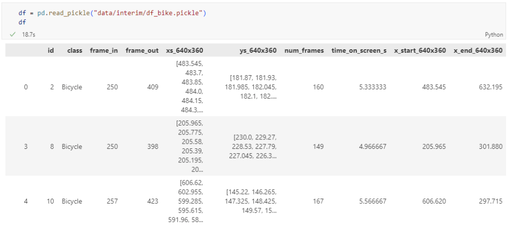
The bicycle trajectory coordinates are stored in two separate lists: xs_640x360 and ys640x360:
This format is kind of similar to the Kaggle Taxi dataset, we worked with in the previous post. However, to use the solution we implemented there, we need to combine the x and y coordinates into nice (x,y) tuples:
Afterwards, we can create the points and compute the proper timestamps from the frame numbers:
def compute_datetime(row):
    # some educated guessing going on here: the paper states that the video covers 2021-06-09 07:00-08:00
    d = datetime(2021,6,9,7,0,0) + (row['frame_in'] + row['running_number']) * timedelta(seconds=2)
    return d
def create_point(xy):
    try:
        return Point(xy)
    except TypeError:  # when there are nan values in the input data
        return None
new_df = df.head().explode('coordinates')
new_df['geometry'] = new_df['coordinates'].apply(create_point)
new_df['running_number'] = new_df.groupby('id').cumcount()
new_df['datetime'] = new_df.apply(compute_datetime, axis=1)
new_df.drop(columns=['coordinates', 'frame_in', 'running_number'], inplace=True)
new_df
Once the points and timestamps are ready, we can create the MovingPandas TrajectoryCollection. Note how we explicitly state that there is no CRS for this dataset (crs=None):
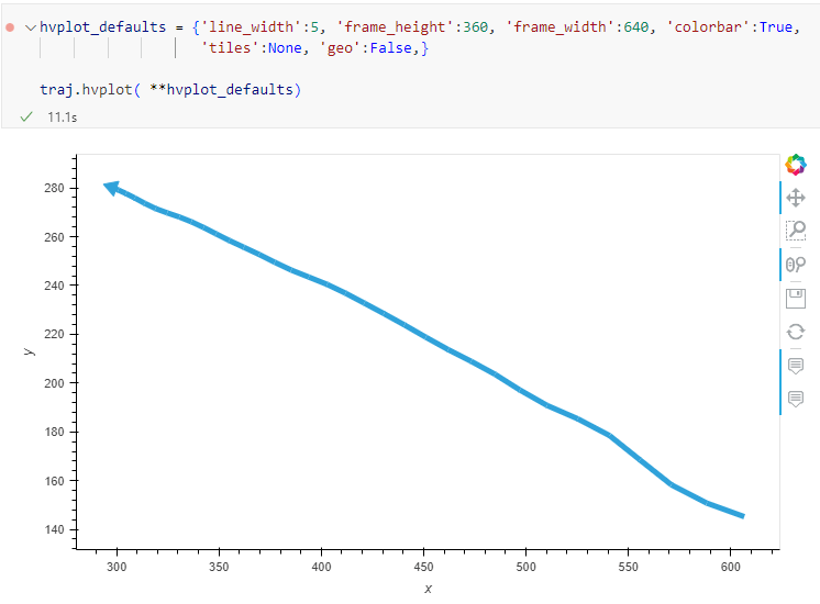
Similarly, to plot these trajectories, we should tell hvplot that it should not fetch any background map tiles (’tiles’:None) and that the coordinates are not geographic (‘geo’:False):
One important caveat is that speed will be calculated in pixels per second. So when we plot the bicycle speed, the segments closer to the camera will appear faster than the segments in the background:
To fix this issue, we would have to correct for the distortions of the camera lens and perspective. I’m sure that there is specialized software for this task but, for the purpose of this post, I’m going to grab the opportunity to finally test out the VectorBender plugin.
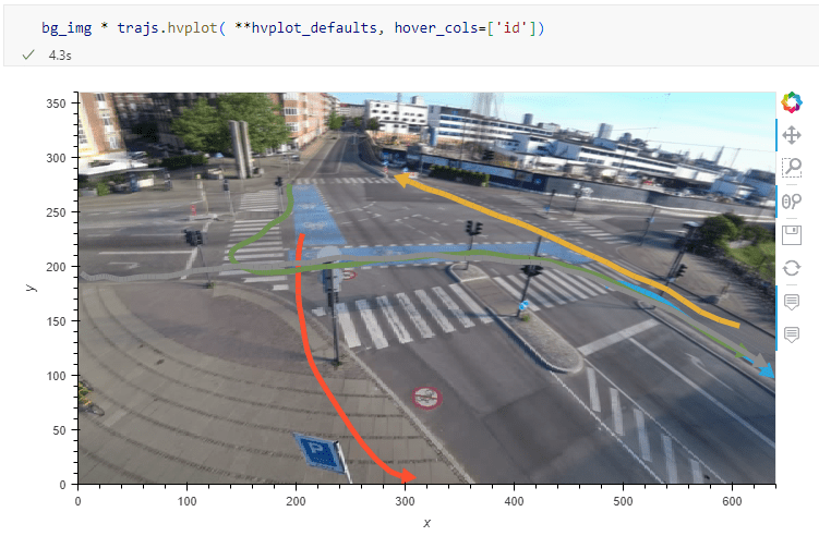
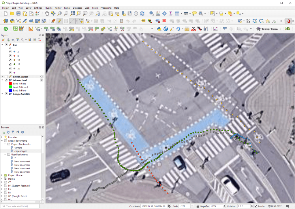
Georeferencing the trajectories using QGIS VectorBender plugin
Let’s load the five test trajectories and the camera image to QGIS. To make sure that they align properly, both are set to the same CRS and I’ve created the following basic world file for the camera image:
1
0
0
-1
0
360
Then we can use the VectorBender tools to georeference the trajectories by linking locations from the camera image to locations on aerial images. You can see the whole process in action here:
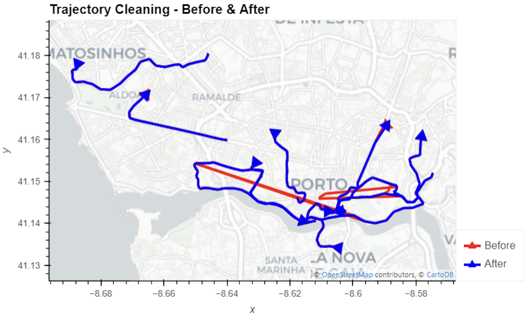
After around 15 minutes linking control points, VectorBender comes up with the following georeferenced trajectory result:
Not bad for a quick-and-dirty hack. Some points on the borders of the image could not be georeferenced since I wasn’t always able to identify suitable control points at the camera image borders. So it won’t be perfect but should improve speed estimates.
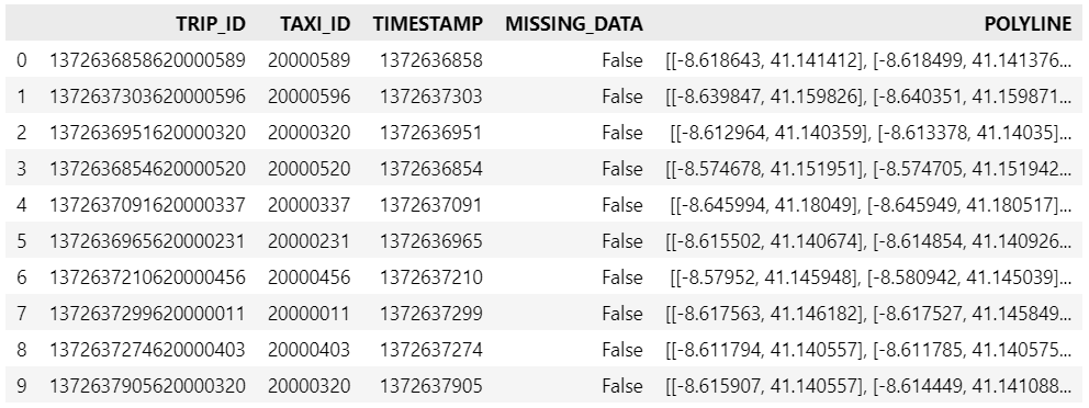
Kaggle’s “Taxi Trajectory Data from ECML/PKDD 15: Taxi Trip Time Prediction (II) Competition” is one of the most used mobility / vehicle trajectory datasets in computer science. However, in contrast to other similar datasets, Kaggle’s taxi trajectories are provided in a format that is not readily usable in MovingPandas since the spatiotemporal information is provided as:
TIMESTAMP: (integer) Unix Timestamp (in seconds). It identifies the trip’s start;
POLYLINE: (String): It contains a list of GPS coordinates (i.e. WGS84 format) mapped as a string. The beginning and the end of the string are identified with brackets (i.e. [ and ], respectively). Each pair of coordinates is also identified by the same brackets as [LONGITUDE, LATITUDE]. This list contains one pair of coordinates for each 15 seconds of trip. The last list item corresponds to the trip’s destination while the first one represents its start;
Therefore, we need to create a DataFrame with one point + timestamp per row before we can use MovingPandas to create Trajectories and analyze them.
But first things first. Let’s download the dataset:
import datetime
import pandas as pd
import geopandas as gpd
import movingpandas as mpd
import opendatasets as od
from os.path import exists
from shapely.geometry import Point

input_file_path = 'taxi-trajectory/train.csv'

def get_porto_taxi_from_kaggle():
    if not exists(input_file_path):
        od.download("https://www.kaggle.com/datasets/crailtap/taxi-trajectory")

get_porto_taxi_from_kaggle()
df = pd.read_csv(input_file_path, nrows=10, usecols=['TRIP_ID', 'TAXI_ID', 'TIMESTAMP', 'MISSING_DATA', 'POLYLINE'])
df.POLYLINE = df.POLYLINE.apply(eval)  # string to list
df
And now for the remodelling:
def unixtime_to_datetime(unix_time):
    return datetime.datetime.fromtimestamp(unix_time)

def compute_datetime(row):
    unix_time = row['TIMESTAMP']
    offset = row['running_number'] * datetime.timedelta(seconds=15)
    return unixtime_to_datetime(unix_time) + offset

def create_point(xy):
    try:
        return Point(xy)
    except TypeError:  # when there are nan values in the input data
        return None

new_df = df.explode('POLYLINE')
new_df['geometry'] = new_df['POLYLINE'].apply(create_point)
new_df['running_number'] = new_df.groupby('TRIP_ID').cumcount()
new_df['datetime'] = new_df.apply(compute_datetime, axis=1)
new_df.drop(columns=['POLYLINE', 'TIMESTAMP', 'running_number'], inplace=True)
new_df
And that’s it. Now we can create the trajectories:
That’s it. Now our MovingPandas.TrajectoryCollection is ready for further analysis.
By the way, the plot above illustrates a new feature in the recent MovingPandas 0.16 release which, among other features, introduced plots with arrow markers that show the movement direction. Other new features include a completely new custom distance, speed, and acceleration unit support. This means that, for example, instead of always getting speed in meters per second, you can now specify your desired output units, including km/h, mph, or nm/h (knots).
These releases are a huge step forward towards making MovingPandas easier to install with fewer mandatory dependencies. All interactive plotting libraries are now optional. So if you are using MovingPandas for trajectory data processing in the background and don’t need the interactive visualization features, the number of necessary libraries is now much lower. This (and the fact that GeoPandas is now shipped with OSGeo4W) will also make it easier to use MovingPandas in QGIS plugins.
We have further improved our repo setup by adding an action that automatically creates and publishes packages from releases, heavily inspired by the work of the GeoPandas team.
Last but not least, we’ve created a Twitter account for the project. (And might soon add a Mastodon account as well.)
As always, all tutorials are available from the movingpandas-examples repository and on MyBinder:
If you have questions about using MovingPandas or just want to discuss new ideas, you’re welcome to join our discussion forum.
New functions to add a timedelta column and get the trajectory sampling interval #233
As always, all tutorials are available from the movingpandas-examples repository and on MyBinder:
The new distance measures are covered in tutorial #11:
Computing distances between trajectories, as illustrated in tutorial #11Computing distances between a trajectory and other geometry objects, as illustrated in tutorial #11
But don’t miss the great features covered by the other notebooks, such as outlier cleaning and smoothing:
Trajectory cleaning and smoothing, as illustrated in tutorial #10
If you have questions about using MovingPandas or just want to discuss new ideas, you’re welcome to join our discussion forum.
Speed and direction column names can now be customized
If you have questions about using MovingPandas or just want to discuss new ideas, you’re welcome to join our recently opened discussion forum.
As always, all tutorials are available from the movingpandas-examples repository and on MyBinder:
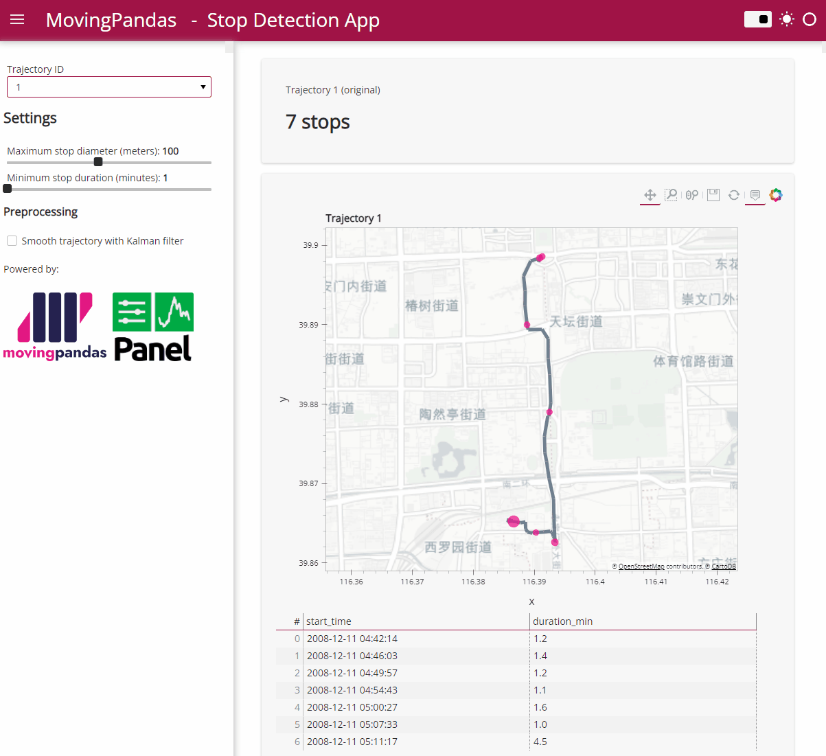
Besides others examples, the movingpandas-examples repo contains the following tech demo: an interactive app built with Panel that demonstrates different MovingPandas stop detection parameters
To start the app, open the stopdetection-app.ipynb notebook and press the green Panel button in the Jupyter Lab toolbar:
The MovingPoint example seems to describe a storm, including its path (temporalGeometry), pressure, wind strength, and class values (temporalProperties):
You can give the current implementation a spin using this MyBinder notebook
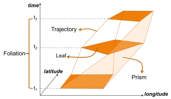
An exciting future step would be to experiment with extending MovingPandas to support the MovingPolygon MF-JSON examples. MovingPolygons can change their size and orientation as they move. I’m not yet sure, however, if the number of polygon nodes can change between time steps and how this would be reflected by the prism concept presented in the draft specification:
First time, we talked about the OGC Moving Features standard in a post from 2017. Back then, we looked at the proposed standard way to encode trajectories in CSV and discussed its issues. Since then, the Moving Features working group at OGC has not been idle. Besides the CSV and XML encodings, they have designed a new JSON encoding that addresses many of the downsides of the previous two. You can read more about this in our 2020 preprint “From Simple Features to Moving Features and Beyond”.
Basically Moving Features JSON (MF-JSON) is heavily inspired by GeoJSON and it comes with a bunch of mandatory and optional key/value pairs. There is support for static properties as well as dynamic temporal properties and, of course, temporal geometries (yes geometries, not just points).
I think this format may have an actual chance of gaining more widespread adoption.
Inspired by Pandas.read_csv() and GeoPandas.read_file(), I’ve started implementing a read_mf_json() function in MovingPandas. So far, it supports basic MovingFeature JSONs with MovingPoint geometry:
You’ll need to use the current development version to test this feature.
Next steps will be MovingFeatureCollection JSONs and support for static as well as temporal properties. We’ll have to see if MovingPandas can be extended to go beyond moving point geometries. Storing moving linestrings and polygons in the GeoDataFrame will be the simple part but analytics and visualization will certainly be more tricky.