Today’s post is a follow-up to a recent map experiment which I published in the QGIS Flickr group. It’s basically an inverted Stamen Toner style with an image in the map composition background instead of a solid color (similar to the approach described for vintage maps):

https://twitter.com/underdarkGIS/status/550340277257650176

That’s nice but with this approach we only get to enjoy the complete design in the print composer but not in the main window. So what other options do we have? – SVG fills to the rescue!

But first we need a suitable SVG with this nice pastel style. I used Gimp to create a seamless version of the pastel image and then embedded the image in an SVG using Inkscape:

In QGIS, this SVG can now be used in any SVG fill. It’s important to set the Texture width setting to a quite high value when working with SVGs containing big textures, otherwise the images will be rendered very small and the repeating patterns will be very obvious.

Once the background is in place, we can add the line work and labels. The roads are white with black outlines for bridges which – together with the Lighten blending mode – produce the desired effect:

Top10 QGIS Planet posts 2014

By underdark

2014-12-27

QGIS

3 Comments

It’s the end of December and time to recap 2014. Therefore, I decided to have a look at what this year has brought us. There were plenty of great posts for both casual and power users as well as developers. Here is my pick of the top 10 posts from the QGIS Planet blog aggregator.

Tons of colour improvements! (Nyall Dawson)
The QGIS Field calculator is dead. Long live the Field calculator bar (Nathan Woodrow)
Why QGIS Class Names Start with Qgs (Gary Sherman)
Atlas Previews (Nyall Dawson)
QGIS atlas on non geometry tables (Nathan Woodrow)
Gradient Fills (Nyall Dawson)
What are all these QGIS file types? Why do I need them (Nathan Woodrow)
Getting Started Writing QGIS Python Plugins (Peter Wells)
QGIS Layer Tree API (Martin Dobias)
Shapeburst fill styles (Nyall Dawson)

More great features and posts are sure to come next year. For example, Nyall is currently running a campaign on Kickstarter to add Live Layer Effects such as drop shadow effects to QGIS. Please support it if you can.

2nd edition of Learning QGIS

By underdark

2014-12-14

QGIS

It’s my pleasure to announce that the updated and extended 2nd edition of Learning QGIS is available now.

I also want to take this opportunity to thank everyone who made the 1st edition such a great success!

This second edition has been updated to QGIS 2.6 and it features a completely new 6th chapter on Expanding QGIS with Python. It introduces the QGIS Python Console, shows how to create custom Processing tools, and provides a starting point for developing plugins.

Overall, the book has grown by 40 pages and the price of the print version has dropped by 3€ :-)

Happy QGISing!

QGIS 2.6 user guide released

By underdark

2014-12-03

QGIS

The QGIS documentations team has released an updated version of the user guide:

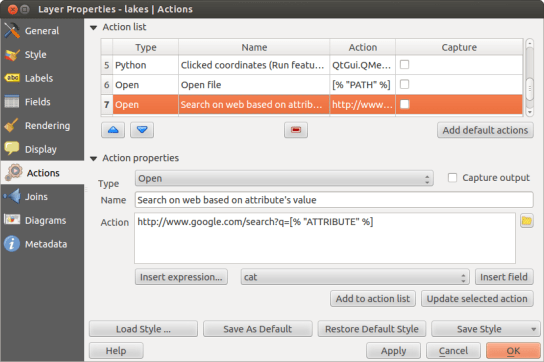
I’d like to encourage everyone to have a look and explore the content, for example the great tips in the Actions menu section:

Analyzing regional income differences

By underdark

2014-11-29

QGIS

8 Comments

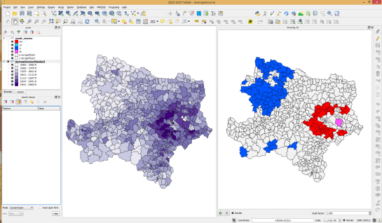
On my quest to create test data for spatial statistics, I’ve discovered income data for Austria per municipality on a news paper website:

For further analysis, I decided to limit the area to Vienna and Lower Austria. Since the income data included GKZ “Gemeindekennzahl” IDs, it was possible to join them to municipalities extracted from OpenStreetMap using QuickOSM for QGIS. GRASS v.clean was used to clean the vector topology to the point where PySAL was able to compute spatial weights.

Using PySAL, I then computed income clusters: blue regions represent low clusters while red regions represent high clusters …

Municipality border data (c) OpenStreetMap and contributors
Income data source: Statistik Austria via derStandard

The results show a statistically significant cluster of low income in the north west, in the area called Waldviertel, as well as a cluster of high income containing many of the municipalities surrounding Vienna, an area often referred to as the “Speckgürtel” (“bacon belt”).

More experiments with Game of Life

By underdark

2014-11-16

QGIS

2 Comments

As promised in my recent post “Experiments with Conway’s Game of Life”, I have been been looking into how to improve my first implementation. The new version which you can now find on Github is fully contained in one Python script which runs in the QGIS console. Additionally, the repository contains a CSV with the grid definition for a Gosper glider gun and the layer style QML.

Rather than creating a new Shapefile for each iteration like in the first implementation, this script uses memory layers to save the game status.

You can see it all in action in the following video:

(video available in HD)

Thanks a lot to Nathan Woodrow for the support in getting the animation running!

Sometimes there are still hick-ups causing steps to be skipped but overall it is running nicely now. Another approach would be to change the layer attributes rather than creating more and more layers but I like to be able to go through all the resulting layers after they have been computed.

Experiments with Conway’s Game of Life

By underdark

2014-11-02

QGIS, Visualization

4 Comments

This experiment is motivated by a discussion I had with Dr. Claus Rinner about introducing students to GIS concepts using Conway’s Game of Life. Conway’s Game of Life is a popular example to demonstrate cellular automata. Based on an input grid of “alive” and “dead” cells, new cell values are computed on each iteration based on four simple rules for the cell and its 8 neighbors:

Any live cell with fewer than two live neighbours dies, as if caused by under-population.
Any live cell with two or three live neighbours lives on to the next generation.
Any live cell with more than three live neighbours dies, as if by overcrowding.
Any dead cell with exactly three live neighbours becomes a live cell, as if by reproduction.

(Source: Wikipedia – Conway’s Game of Life)

Based on these simple rules, effects like the following “glider gun” can be achieved:

“Gospers glider gun” by Kieff – Own work. Licensed under CC BY-SA 3.0 via Wikimedia Commons.

There are some Game of Life implementations for GIS out there, e.g. scripts for ArcGIS or a module for SAGA. Both of these examples are raster-based. Since I couldn’t find any examples of raster manipulation like this in pyQGIS, I decided to instead implement a vector version: a Processing script which receives an input grid of cells and outputs the next iteration based on the rules of Game of Life. In the following screencast, you can see the Processing script being called repeatedly by a script from the Python console:

So far, it’s a quick and dirty first implementation. To make it more smooth, I’m considering adding spatial indexing and using memory layers instead of having Processing create a bunch of Shapefiles.

It would also be interesting to see a raster version done in PyQGIS. Please leave a comment if you have any ideas how this could be achieved.

Labels as text in SVG exports

By underdark

2014-09-20

QGIS

3 Comments

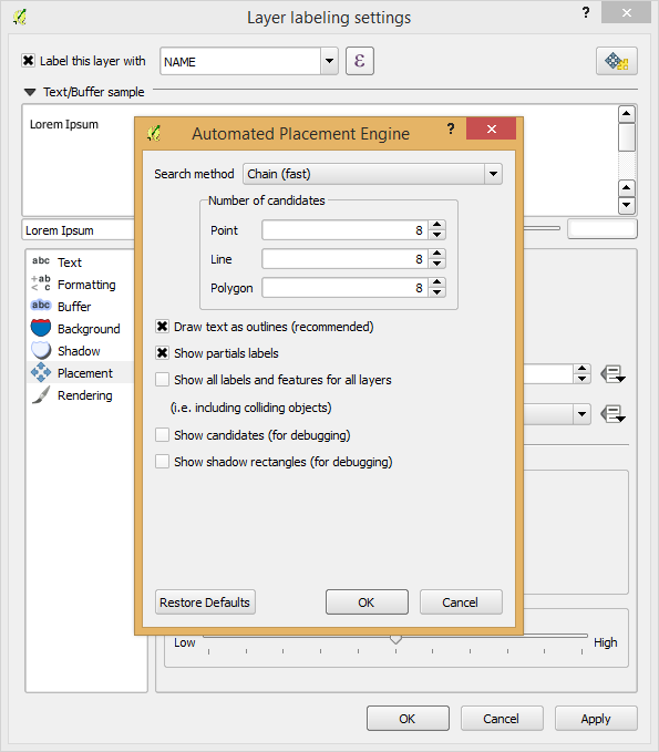
Today’s post is inspired by a recent thread on the QGIS user mailing list titled “exporting text to Illustrator?”. The issue was that with the introduction of the new labeling system, all labels were exported as paths when creating an SVG. Unnoticed by almost everyone (and huge thanks to Alex Mandel for pointing out!) an option has been added to 2.4 by Larry Shaffer which allows exporting labels as texts again.

To export labels as text, open the Automatic Placement Settings (button in the upper right corner of the label dialog) and uncheck the Draw text as outlines option.

Note that we are also cautioned that

For now the developers recommend you only toggle this option right
before exporting and that you recheck it after.

Alex even recorded a video showcasing the functionality:

Visualizing direction-dependent values

By underdark

2014-07-21

GIS, QGIS

7 Comments

When mapping flows or other values which relate to a certain direction, styling these layers gets interesting. I faced the same challenge when mapping direction-dependent error values. Neighboring cell pairs were connected by two lines, one in each direction, with an associated error value. This is what I came up with:

Each line is drawn with an offset to the right. The size of the offset depends on the width of the line which in turn depends on the size of the error. You can see the data-defined style properties here:

To indicate the direction, I added a marker line with one > marker at the center. This marker line also got assigned the same offset to match the colored line bellow. I’m quite happy with how these turned out and would love to hear about your approaches to this issue.

These figures are part of a recent publication with my AIT colleagues: A. Graser, J. Asamer, M. Dragaschnig: “How to Reduce Range Anxiety? The Impact of Digital Elevation Model Quality on Energy Estimates for Electric Vehicles” (2014).

Toner-lite styles for QGIS

By underdark

2014-06-07

Cartography, OSM, QGIS

2 Comments

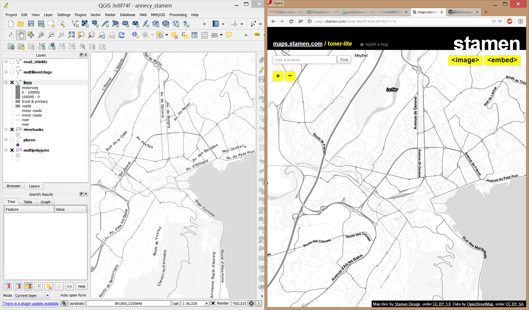
In my opinion, Stamen’s Toner-lite map is one of the best background maps to use together with colorful overlays. The only downsides of using it in QGIS are that the OpenLayers plugin can not provide the tiles at print resolution and that the projection is limited to Web Mercator. That’s why I’ve started to recreate the style for OSM Spatialite databases:

So far, there are styles for lines and polygons and they work quite well for the scale range between 1:1 and 1:250000. As always, you can download the styles from QGIS-resources on Github.