We are celebrating FOSS4G 2015 in Seoul with great open source GIS book discounts at both Packt and Locate Press. So if you don’t have a copy of “Learning QGIS”, “The PyQGIS Programmer’s Guide”, or “Geospatial Power Tools” yet, check out the following sites:
This is a guest post by Karolina Alexiou (aka carolinux), Anita’s collaborator on the Time Manager plugin.
As of version 2.1.5, TimeManager provides some support for stepping through WMS-T layers, a format about which Anita has written in the past. From the official definition, the OpenGIS® Web Map Service Interface Standard (WMS) provides a simple HTTP interface for requesting geo-registered map images from one or more distributed geospatial databases. A WMS request defines the geographic layer(s) and area of interest to be processed. The response to the request is one or more geo-registered map images (returned as JPEG, PNG, etc) that can be displayed in a browser application. QGIS can display those images as a raster layer. The WMS-T standard allows the user of the service to set a time boundary in addition to a geographical boundary with their HTTP request.
From QGIS, go to Layer>Add Layer>Add WMS/WMST Layer and add a new server and connect to it. For the service we have chosen, we only need to specify a name and the url.
Select the top level layer, in our case named nexrad_base_reflect and click Add. Now you have added the layer to your QGIS project.
To add it to TimeManager as well, add it as a raster with the settings from the screenshot below. Start time and end time have the values 2005-08-29T03:10:00Z and 2005-08-30T03:10:00Z respectively, which is a period which overlaps with hurricane Katrina. Now, the WMS-T standard uses a handful of different time formats, and at this time, the plugin requires you to know this format and input the start and end values in this format. If there’s interest to sponsor this feature, in the future we may get the format directly from the web service description. The web service description is an XML document (see here for an example) which, among other information, contains a section that defines the format, default time and granularity of the time dimension.
If we set the time step to 2 hours and click play, we will see that TimeManager renders each interval by querying the web map service for it, as you can see in this short video.
Querying the web service and waiting for the response takes some time. So, the plugin requires some patience for looking at this particular layer format in interactive mode. If we export the frames, however, we can get a nice result. This is an animation showing hurricane Katrina progressing over a 30 minute interval.
If you want to sponsor further development of the Time Manager plugin, you can arrange a session with me – Karolina Alexiou – via Codementor.
This is a follow-up on my previous post introducing an Open source IDF parser for QGIS. Today’s post takes the code further and adds routing functionality for foot, bike, and car routes including oneway streets and turn restrictions.
You can find the script in my QGIS-resources repository on Github. It creates an IDFRouter object based on an IDF file which you can use to compute routes.
The following screenshot shows an example car route in Vienna which gets quite complex due to driving restrictions. The dark blue line is computed by my script on GIP data while the light blue line is the route from OpenRouteService.org (via the OSM route plugin) on OSM data. Minor route geometry differences are due to slight differences in the network link geometries.
IDF is the data format used by Austrian authorities to publish the official open government street graph. It’s basically a text file describing network nodes, links, and permissions for different modes of transport.
I haven’t implemented all details yet but it successfully parses nodes and links from the two example IDF files that have been published so far as can be seen in the following screenshot which shows the Klagenfurt example data:
If you are interested in advancing this project, just get in touch here or on Github.
If you follow my blog, you’ve most certainly seen the post How to create illuminated contours, Tanaka-style from earlier this year. As Victor Olaya noted correctly in the comments, the workflow to create this effect lends itself perfectly to being automated with a Processing model.
The model needs only two inputs: the digital elevation model raster and the interval at which we want the contours to be created:
The model steps are straightforward: the contours are generated and split into short segments before the segment orientation is computed using the following code in the Advanced Python Field Calculator:
p1 = $geom.asPolyline()[0]
p2 = $geom.asPolyline()[-1]
a = p1.azimuth(p2)
if a < 0:
   a += 360
value = a
It’s my pleasure to report back from this year’s AGIT and GI_Forum conference (German and English speaking respectively). It was great to meet the gathered GIS crowd! If you missed it, don’t despair: I’ve compiled a personal summary on Storify, and papers (German, English) and posters are available online. Here’s a pick of my favorite posters:
I also had the pleasure to be involved in multiple presentations this year:
QGIS at the OSGeo Day
As part of the OSGeo Day, I had the chance to present the latest and greatest QGIS features for map design in front of a full house:
On a slightly different note, my colleague Markus Straub and I presented an introduction to routing with OpenStreetMap covering which kind of routing-related information is available in OSM as well as a selection of different tools to perform routing on OSM.
Solving the “unnamed link” problem
In this talk, I presented approaches to solving issues with route descriptions that contain unnamed pedestrian or cycle paths.
In this talk, my colleague Markus Straub presented our new approach to computing how popular a certain road is. The resulting popularity value can be used for planning as well as routing.
With the release of 2.10 right around the corner, it’s time to have a look at the new features this version of QGIS will bring. One area which has received a lot of development attention is layer styling. In particular, I want to point out the following new features:
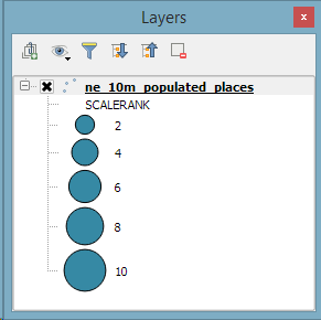
1. Graduated symbol size
The graduated renderer has been expanded. Formerly, only color-graduated symbols could be created automatically. Now, it is possible to choose between color and size-graduated styles:
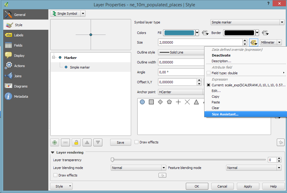
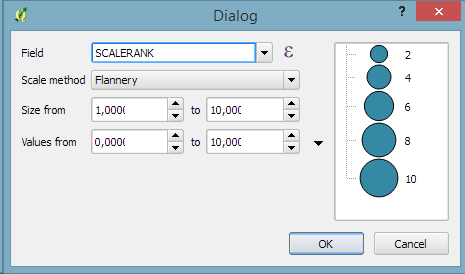
2. Symbol size assistant
On a similar note, I’m sure you’ll enjoy the size assistant for data-defined size:
What’s particularly great about this feature is that it also creates a proper legend for the data-defined sizes:
3. Interactive class exploration and definition
Another great addition to the graduated renderer dialog is the histogram tab which visualizes the distribution of values as well as the defined class borders. Additionally, the user can interactively change the classes by moving the class borders:
If you follow the QGIS developer mailing list, you’ve probably seen threads about the next major release: 3.0. The topic has been one of the many points we talked about at the latest QGIS developer meeting and Tim Sutton sums up the discussed plan in a post published today:
One hot topic was ‘when will QGIS 3.0 be released’. The short answer to that question is that ‘we don’t know’ – Jürgen Fischer and Matthias Kuhn are still investigating our options and once they have had enough time to understand the implications of upgrading to Qt5, Python 3 etc. they will make some recommendations. I can tell you that we agreed to announce clearly and long in advance (e.g. 1 year) the roadmap to moving to QGIS 3.0 so that plugin builders and others who are using QGIS libraries for building third party apps will have enough time to be ready for the transition. At the moment it is still uncertain if there even is a pressing need to make the transition, so we are going to hang back and wait for Jürgen & Matthias’ feedback.
The take-away message here is that the QGIS team is aware of the current developments around Python and Qt and will keep the community updated about the further development path well before any move.