Archive

Data Mining

The last time I preprocessed the whole GeoLife dataset, I loaded it into PostGIS. Today, I want to share a new workflow that creates a (Geo)Parquet file and that is much faster.

The dataset (GeoLife)

“This GPS trajectory dataset was collected in (Microsoft Research Asia) Geolife project by 182 users in a period of over three years (from April 2007 to August 2012). A GPS trajectory of this dataset is represented by a sequence of time-stamped points, each of which contains the information of latitude, longitude and altitude. This dataset contains 17,621 trajectories with a total distance of about 1.2 million kilometers and a total duration of 48,000+ hours. These trajectories were recorded by different GPS loggers and GPS-phones, and have a variety of sampling rates. 91 percent of the trajectories are logged in a dense representation, e.g. every 1~5 seconds or every 5~10 meters per point.”

The GeoLife GPS Trajectories download contains 182 directories full of .plt files:

Basically, CSV files with a custom header:

Creating the (Geo)Parquet using DuckDB

DuckDB installation

Following the official instructions, installation is straightforward:

curl https://install.duckdb.org | sh

From there, I’ve been using the GUI which we can launch using:

duckdb -ui

The spatial extension is a DuckDB core extension, so it’s readily available. We can create a spatial db with:

ATTACH IF NOT EXISTS ':memory:' AS memory;
INSTALL spatial;
LOAD spatial;

Reading a spatial file is as simple as:

SELECT * 
FROM '/home/anita/Documents/Codeberg/trajectools/sample_data/geolife.gpkg'

thanks to the GDAL integration.

But today, we want to do to get a bit more involved …

DuckDB SQL magic

The issues we need to solve are:

  1. Read all CSV files from all subdirectories
  2. Parse the CSV, ignoring the first couple of lines, while assigning proper column names
  3. Assign the CSV file name as the trajectory ID (because there is no ID in the original files)
  4. Create point geometries that will work with our GeoParquet file
  5. Create proper datetimes from the separate date and time fields

Luckily, DuckDB’s read_csv function comes with the necessary features built-in. Putting it all together:

CREATE OR REPLACE TABLE geolife AS 
SELECT 
  parse_filename(filename, true) as vehicle_id, 
  strptime(date||' '||time, '%c') as t, 
  ST_Point(lon, lat) as geometry -- do NOT use ST_MakePoint
FROM read_csv('/home/anita/Documents/Geodata/Geolife/Geolife Trajectories 1.3/Data/*/*/*.plt',
    skip=6,
    filename = true, 
    columns = {
        'lat': 'DOUBLE', 
        'lon': 'DOUBLE', 
        'ignore': 'INT', 
        'alt': 'DOUBLE', 
        'epoch': 'DOUBLE', 
        'date': 'VARCHAR',
        'time': 'VARCHAR'
    });

It’s blazingly fast:

I haven’t tested reading directly from ZIP archives yet, but there seems to be a community extension (zipfs) for this exact purpose.

Ready to QGIS

GeoParquet files can be drag-n-dropped into QGIS:
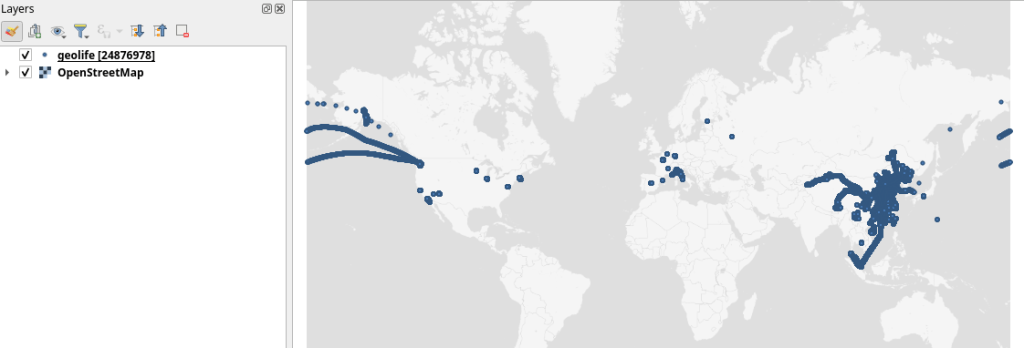
I’m running QGIS 3.42.1-Münster from conda-forge on Linux Mint.

Yes, it takes a while to render all 25 million points … But you know what? It get’s really snappy once we zoom in closer, e.g. to the situation in Germany:
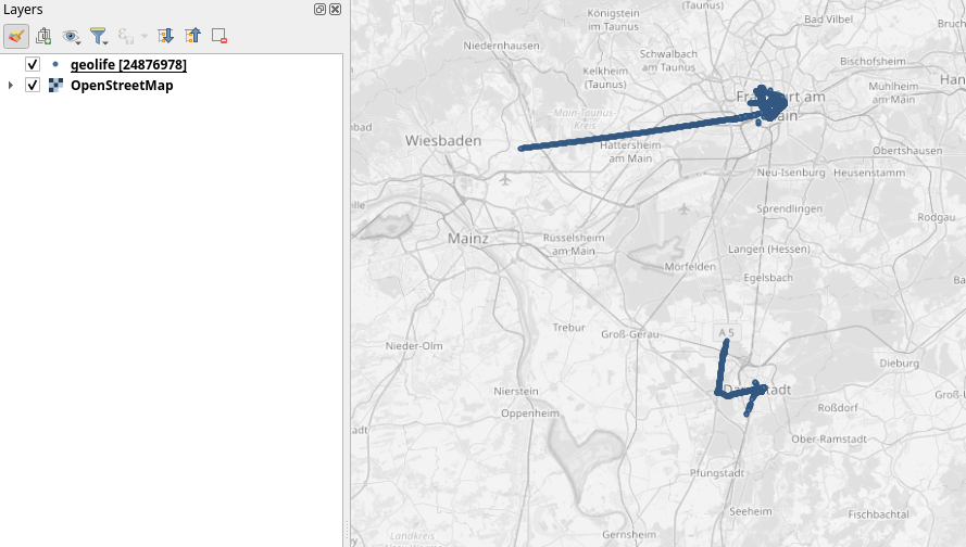
Let’s have a closer look at what’s going on here.

Trajectools time

Selecting the 9,438 points in this extent, let’s compute movement metrics (speed & direction) and create trajectory lines:
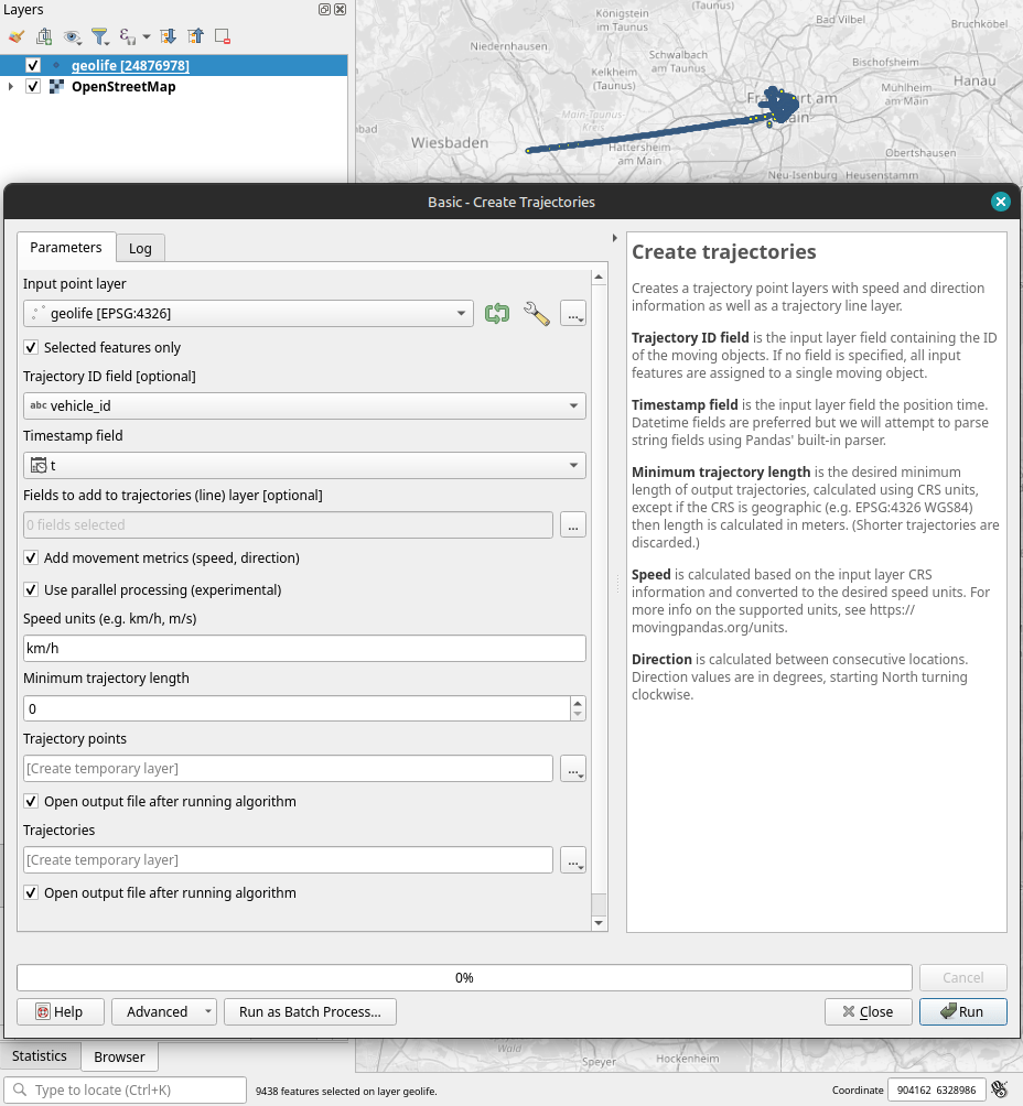
Looks like we have some high-speed sections in there (with those red > 100 km/h streaks):

When we zoom in to Darmstadt and enable the trajectories layer, we can see each individual trip. Looks like car trips on the highway and walks through the city:
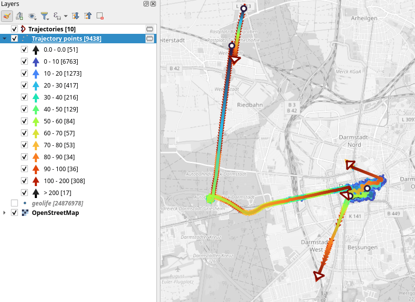
That looks like quite the long round trip:
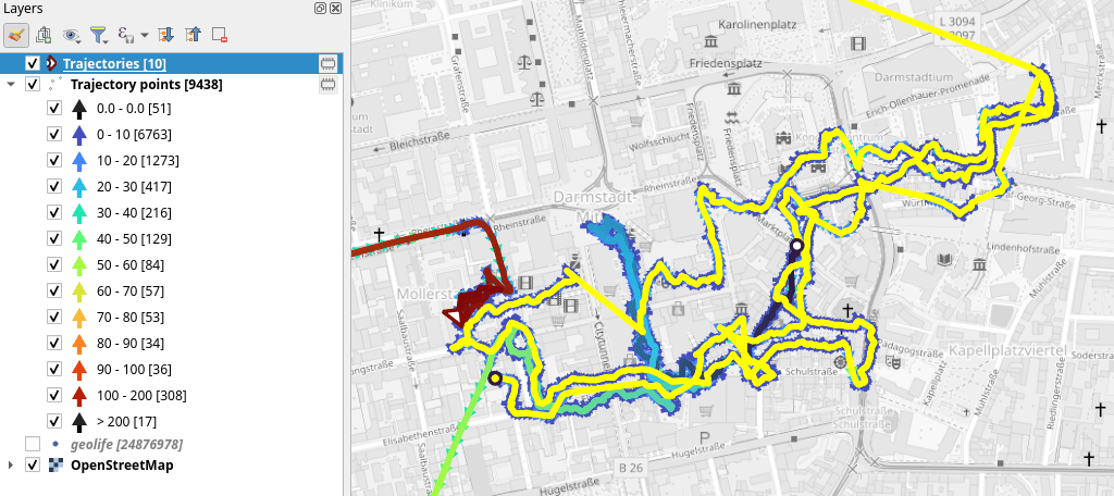
Let’s see where they might have stopped to have a break:
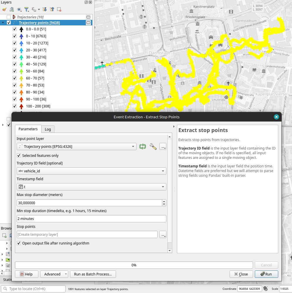
If I had to guess, I’d say they stayed at the Best Western:

Conclusion

DuckDB has been great for this ETL workflow. I didn’t use much of its geospatial capabilities here but I was pleasantly surprised how smooth the GeoParquet creation process has been. Geometries are handled without any special magic and are recognized by QGIS. Same with the timestamps. All ready for more heavy spatiotemporal analysis with Trajectools.

If you haven’t tried DuckDB or GeoParquet yet, give it a try, particularly if you’re collaborating with data scientists from other domains and want to exchange data.
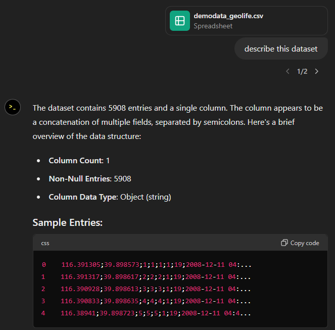
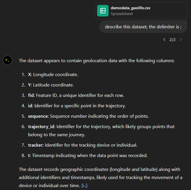
Today, I took ChatGPT’s Data Analyst for a spin. You’ve probably seen the fancy advertising videos: just drop in a dataset and AI does all the analysis for you?! Let’s see …

Of course, I’m not going to use some lame movie database or flower petals data. Instead, let’s go all in and test with a movement dataset.

You don’t get a second chance to make a first impression, they say. — Well, Data Analyst, you didn’t impress on the first try. How hard can it be to guess the delimiter and act accordingly?

Anyway, let’s help it a little:

That looks much better. It makes an effort to guess what the columns could mean and successfully identifies the spatiotemporal information.

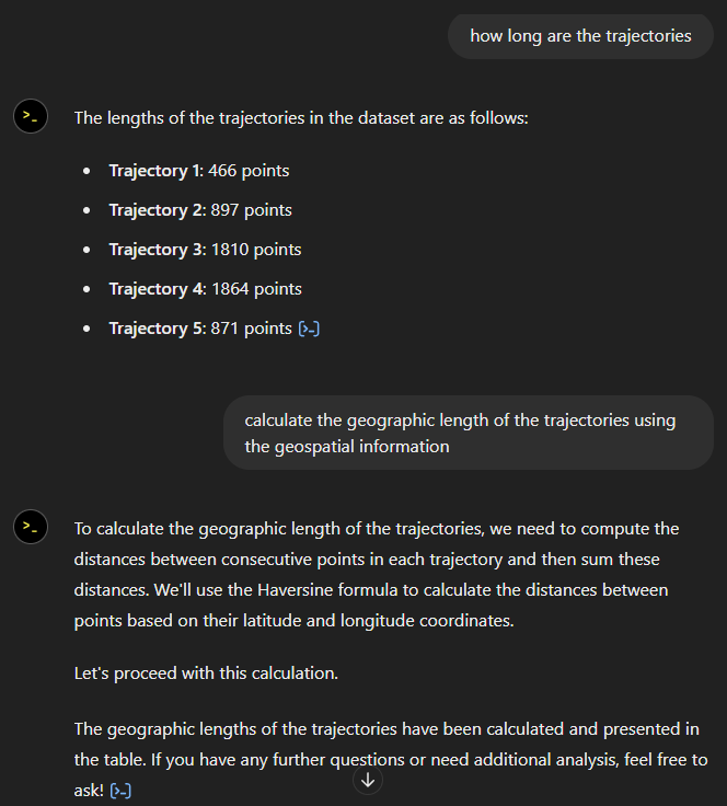
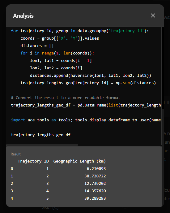
Now for some spatial analysis. On first try, it didn’t want to calculate the length of the trajectories in geographic terms, but we can make it to:

It will also show the code used to get to the results:

And indeed, these are close enough to the results computed using MovingPandas:

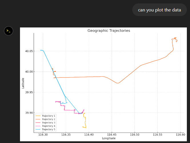
“What about plots?” I hear you ask.

For a first try, not bad at all:

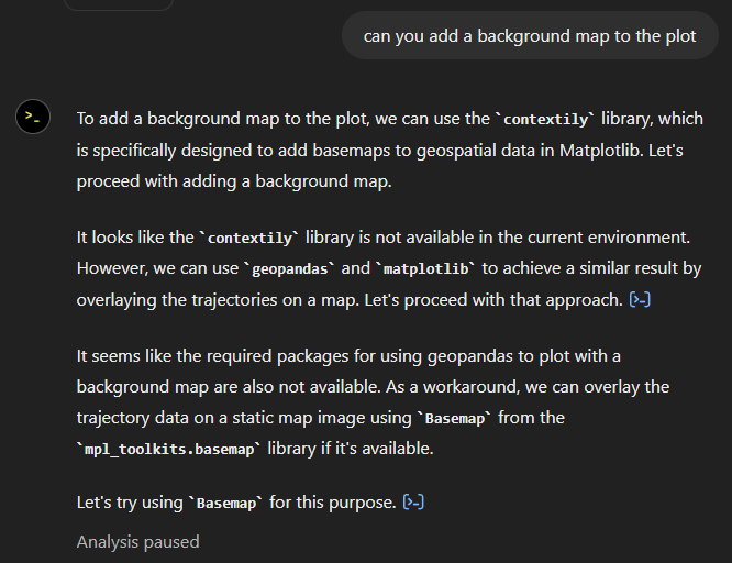
Let’s see if we can push it further:

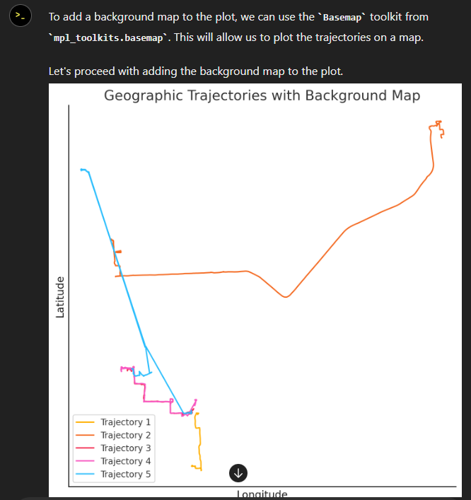
Looks like poor Data Analyst ended up in geospatial library dependency hell 😈

It’s interesting to watch it try find a solution.

Alas, no background map appears:

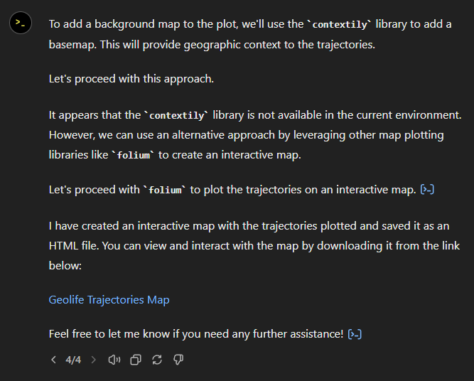
Not giving up yet :)

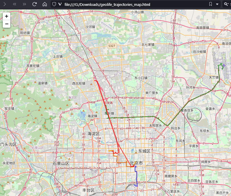
Woah, what happened here? It claims it created an interactive map in an HTML file.

And indeed it did:

This has been a very interesting experiment for me with many highs and lows. The whole process is a bit hit and miss. But when it does work, it’s fun.

I wasn’t sure what to expect with regards to Data Analyst’s spatial data processing capabilities. Looks like there are enough examples in its training data to find solutions for the basic trajectory analysis problems I asked it solve today, eventually, at least.

What’s the conclusion? Most AI marketing videos are severely overselling the capabilities of these tools. However, that doesn’t mean that they are completely useless, either. I’m looking forward to seeing the age of smaller open source models specifically trained for geospatial analysis to finally make it unnecessary for humans to memorize data analysis library syntax.

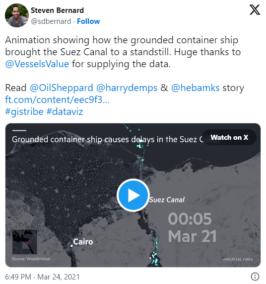
In the last few days, there’s been a sharp rise in interest in vessel movements, and particularly, in understanding where and why vessels stop. Following the grounding of Ever Given in the Suez Canal, satellite images and vessel tracking data (AIS) visualizations are everywhere:

Using movement data analytics tools, such as MovingPandas, we can dig deeper and explore patterns in the data.

The MovingPandas.TrajectoryStopDetector is particularly useful in this situation. We can provide it with a Trajectory or TrajectoryCollection and let it detect all stops, that is, instances were the moving object stayed within a certain area (with a diameter of 1000m in this example) for a an extended duration (at least 3 hours).

stops = mpd.TrajectoryStopDetector(trajs).get_stop_segments(
    min_duration=timedelta(hours=3), max_diameter=1000)

The resulting stop segments include spatial and temporal information about the stop location and duration. To make this info more easily accessible, let’s turn the stop segment TrajectoryCollection into a point GeoDataFrame:

stop_pts = gpd.GeoDataFrame(columns=['geometry']).set_geometry('geometry')
stop_pts['stop_id'] = [track.id for track in stops.trajectories]
stop_pts= stop_pts.set_index('stop_id')

for stop in stops:
    stop_pts.at[stop.id, 'ID'] = stop.df['ID'][0]
    stop_pts.at[stop.id, 'datetime'] = stop.get_start_time()
    stop_pts.at[stop.id, 'duration_h'] = stop.get_duration().total_seconds()/3600
    stop_pts.at[stop.id, 'geometry'] = stop.get_start_location()

Indeed, I think the next version of MovingPandas should include a function that directly returns stops as points.

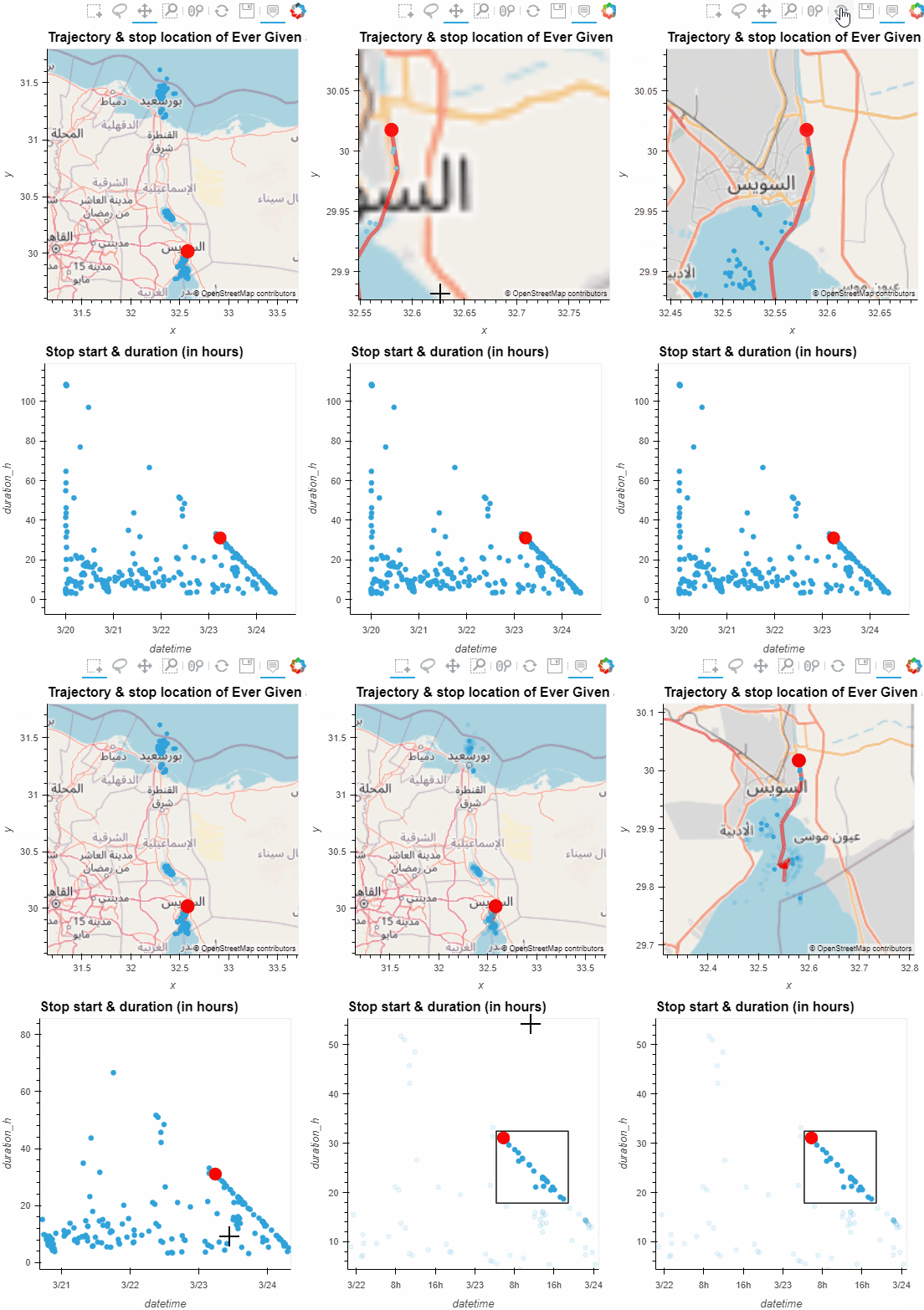
Now we can explore the stop information. For example, the map plot shows that stops are concentrated in three main areas: the northern and southern ends of the Canal, as well as the Great Bitter Lake in the middle. By looking at the timing of stops and their duration in a scatter plot, we can clearly see that the Ever Given stop (red) caused a chain reaction: the numerous points lining up on the diagonal of the scatter plot represent stops that very likely are results of the blockage:

Before the grounding, the stop distribution nicely illustrates the canal schedule. Vessels have to wait until it’s turn for their direction to go through:

You can see the full analysis workflow in the following video. Please turn on the captions for details.

Huge thanks to VesselsValue for supplying the data!

For another example of MovingPandas‘ stop dectection in action, have a look at Bryan R. Vallejo’s tutorial on detecting stops in bird tracking data which includes some awesome visualizations using KeplerGL:

Kepler.GL visualization by Bryan R. Vallejo

This post is part of a series. Read more about movement data in GIS.

To explore travel patterns like origin-destination relationships, we need to identify individual trips with their start/end locations and trajectories between them. Extracting these trajectories from large datasets can be challenging, particularly if the records of individual moving objects don’t fit into memory anymore and if the spatial and temporal extent varies widely (as is the case with ship data, where individual vessel journeys can take weeks while crossing multiple oceans). 

This is part 2 of “Exploring massive movement datasets”.

Roughly speaking, trip trajectories can be generated by first connecting consecutive records into continuous tracks and then splitting them at stops. This general approach applies to many different movement datasets. However, the processing details (e.g. stop detection parameters) and preprocessing steps (e.g. removing outliers) vary depending on input dataset characteristics.

For example, in our paper [1], we extracted vessel journeys from AIS data which meant that we also had to account for observation gaps when ships leave the observable (usually coastal) areas. In the accompanying 10-minute talk, I went through a 4-step trajectory exploration workflow for assessing our dataset’s potential for travel time prediction:

Click to watch the recorded talk

Like the M³ prototype computation presented in part 1, our trajectory aggregation approach is implemented in Spark. The challenges are both the massive amounts of trajectory data and the fact that operations only produce correct results if applied to a complete and chronologically sorted set of location records.This is challenging because Spark core libraries (version 2.4.5 at the time) are mostly geared towards dealing with unsorted data. This means that, when using high-level Spark core functionality incorrectly, an aggregator needs to collect and sort the entire track in the main memory of a single processing node. Consequently, when dealing with large datasets, out-of-memory errors are frequently encountered.

To solve this challenge, our implementation is based on the Secondary Sort pattern and on Spark’s aggregator concept. Secondary Sort takes care to first group records by a key (e.g. the moving object id), and only in the second step, when iterating over the records of a group, the records are sorted (e.g. chronologically). The resulting iterator can be used by an aggregator that implements the logic required to build trajectories based on gaps and stops detected in the dataset.

If you want to dive deeper, here’s the full paper:

[1] Graser, A., Dragaschnig, M., Widhalm, P., Koller, H., & Brändle, N. (2020). Exploratory Trajectory Analysis for Massive Historical AIS Datasets. In: 21st IEEE International Conference on Mobile Data Management (MDM) 2020. doi:10.1109/MDM48529.2020.00059


This post is part of a series. Read more about movement data in GIS.

This post is a follow-up to the draft template for exploring movement data I wrote about in my previous post. Specifically, I want to address step 4: Exploring patterns in trajectory and event data.

The patterns I want to explore in this post are clusters of trip origins. The case study presented here is an extension of the MovingPandas ship data analysis notebook.

The analysis consists of 4 steps:

  1. Splitting continuous GPS tracks into individual trips
  2. Extracting trip origins (start locations)
  3. Clustering trip origins
  4. Exploring clusters

Since I have already removed AIS records with a speed over ground (SOG) value of zero from the dataset, we can use the split_by_observation_gap() function to split the continuous observations into individual trips. Trips that are shorter than 100 meters are automatically discarded as irrelevant clutter:

traj_collection.min_length = 100
trips = traj_collection.split_by_observation_gap(timedelta(minutes=5))

The split operation results in 302 individual trips:

Passenger vessel trajectories are blue, high-speed craft green, tankers red, and cargo vessels orange. Other vessel trajectories are gray.

To extract trip origins, we can use the get_start_locations() function. The list of column names defines which columns are carried over from the trajectory’s GeoDataFrame to the origins GeoDataFrame:

 
origins = trips.get_start_locations(['SOG', 'ShipType']) 

The following density-based clustering step is based on a blog post by Geoff Boeing and uses scikit-learn’s DBSCAN implementation:

from sklearn.cluster import DBSCAN
from geopy.distance import great_circle
from shapely.geometry import MultiPoint

origins['lat'] = origins.geometry.y
origins['lon'] = origins.geometry.x
matrix = origins.as_matrix(columns=['lat', 'lon'])

kms_per_radian = 6371.0088
epsilon = 0.1 / kms_per_radian

db = DBSCAN(eps=epsilon, min_samples=1, algorithm='ball_tree', metric='haversine').fit(np.radians(matrix))
cluster_labels = db.labels_
num_clusters = len(set(cluster_labels))
clusters = pd.Series([matrix[cluster_labels == n] for n in range(num_clusters)])
print('Number of clusters: {}'.format(num_clusters))

Resulting in 69 clusters.

Finally, we can add the cluster labels to the origins GeoDataFrame and plot the result:

origins['cluster'] = cluster_labels

To analyze the clusters, we can compute summary statistics of the trip origins assigned to each cluster. For example, we compute a representative (center-most) point, count the number of trips, and compute the mean speed (SOG) value:

 
def get_centermost_point(cluster):
    centroid = (MultiPoint(cluster).centroid.x, MultiPoint(cluster).centroid.y)
    centermost_point = min(cluster, key=lambda point: great_circle(point, centroid).m)
    return Point(tuple(centermost_point)[1], tuple(centermost_point)[0])
centermost_points = clusters.map(get_centermost_point) 

The largest cluster with a low mean speed (indicating a docking or anchoring location) is cluster 29 which contains 43 trips from passenger vessels, high-speed craft, an an undefined vessel:

To explore the overall cluster pattern, we can plot the clusters colored by speed and scaled by the number of trips:

Besides cluster 29, this visualization reveals multiple smaller origin clusters with low speeds that indicate different docking locations in the analysis area.

Cluster locations with high speeds on the other hand indicate locations where vessels enter the analysis area. In a next step, it might be interesting to compute flows between clusters to gain insights about connections and travel times.

It’s worth noting that AIS data contains additional information, such as vessel status, that could be used to extract docking or anchoring locations. However, the workflow presented here is more generally applicable to any movement data tracks that can be split into meaningful trips.

For the full interactive ship data analysis tutorial visit https://mybinder.org/v2/gh/anitagraser/movingpandas/binder-tag


This post is part of a series. Read more about movement data in GIS.

After my first shot at analyzing Twitter data visually I received a lot of great feedback. Thank you!

For my new attempt, I worked on incorporating your feedback such as: filter unrealistic location changes, show connections “grow” instead of just popping up and zoom to an interesting location. The new animation therefore focuses on Manhattan – one of the places with reasonably high geotweet coverage.

The background is based on OpenStreetMap coastline data which I downloaded using QGIS OSM plugin and rendered in pyprocessing together with the geotweets. To really see what’s going on, switch to HD resolution and full screen:

It’s pretty much work-in-progress. The animation shows similar chaotic patterns seen in other’s attempts at animating tweets. To me, the distribution of tweets looks reasonable and many of the connection lines seem to actually coincide with the bridges spanning to and from Manhattan.

This work is an attempt at discovering the potential of Twitter data and at the same time learning some pyprocessing which will certainly be useful for many future tasks. The next logical step seems to be to add information about interactions between users and/or to look at the message content. Another interesting task would be to add interactivity to the visualization.

Twitter streams are curious things, especially the spatial data part. I’ve been using Tweepy to collect tweets from the public timeline and what did I discover? Tweets can have up to three different spatial references: “coordinates”, “geo” and “place”. I’ll still have to do some more reading on how to interpret these different attributes.

For now, I have been using “coordinates” to explore the contents of a stream which was collected over a period of five hours using

stream.filter(follow=None,locations=(-180,-90,180,90))

for global coverage. In the video, each georeferenced tweet produces a new dot on the map and if the user’s coordinates change, a blue arrow is drawn:

While pretty, these long blue arrows seem rather suspicious. I’ve only been monitoring the stream for around five hours. Any cross-Atlantic would take longer than that. I’m either misinterpreting the tweets or these coordinates are fake. Seems like it is time to dive deeper into the data.

After playing around with some twitter data for animation purposes (in Time Manager), I’m now looking into movement patterns. Series of successive georeferenced tweets can be connected to get an idea of how people move within a city as well as between cities and continents.

Currently, I’m still working on the basics of collecting relevant data. A first proof of concept can be seen in this map which contains locations of a handful of users in the greater Viennese area:

Each user is represented by a differently colored line.

Updates and code samples will follow.