Today marks the 2.1 release of Trajectools for QGIS. This release adds multiple new algorithms and improvements. Since some improvements involve upstream MovingPandas functionality, I recommend to also update MovingPandas while you’re at it.
If you have installed QGIS and MovingPandas via conda / mamba, you can simply:
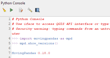
Afterwards, you can check that the library was correctly installed using:
import movingpandas as mpd
mpd.show_versions()
Trajectools 2.1
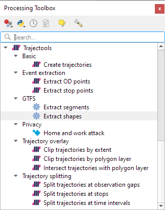
The new Trajectools algorithms are:
Trajectory overlay — Intersect trajectories with polygon layer
Privacy — Home work attack (requires scikit-mobility)
This algorithm determines how easy it is to identify an individual in a dataset. In a home and work attack the adversary knows the coordinates of the two locations most frequently visited by an individual.
Furthermore, we have fixed issue with previously ignored minimum trajectory length settings.
Scikit-mobility and gtfs_functions are optional dependencies. You do not need to install them, if you do not want to use the corresponding algorithms. In any case, they can be installed using mamba and pip:
I’m continuously testing the algorithms integrated so far to see if they work as GIS users would expect and can to ensure that they can be integrated in Processing model seamlessly.
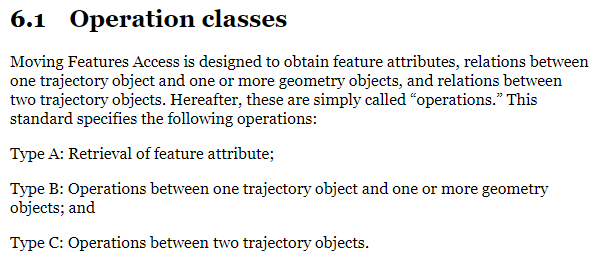
Because naming things is tricky, I’m currently struggling with how to best group the toolbox algorithms into meaningful categories. I looked into the categories mentioned in OGC Moving Features Access but honestly found them kind of lacking:
… but I’m not convinced yet. So take the above listed three categories with a grain of salt. Those may change before the release. (Any inputs / feedback / recommendation welcome!)
Let me close this quick status update with a screencast showcasing stop detection in AIS data, featuring the recently added trajectory styling using interpolated lines:
Then we can connect to our database. The default user name is neo4j and you get to pick the password when creating the database:
from neo4j import GraphDatabase

URI = "neo4j://localhost"
AUTH = ("neo4j", "password")

with GraphDatabase.driver(URI, auth=AUTH) as driver:
    driver.verify_connectivity()
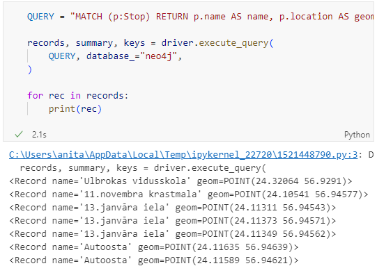
Once we have confirmed that the connection works as expected, we can run a query:
QUERY = "MATCH (p:Stop) RETURN p.name AS name, p.location AS geom"

records, summary, keys = driver.execute_query(
    QUERY, database_="neo4j",
)

for rec in records:
    print(rec)
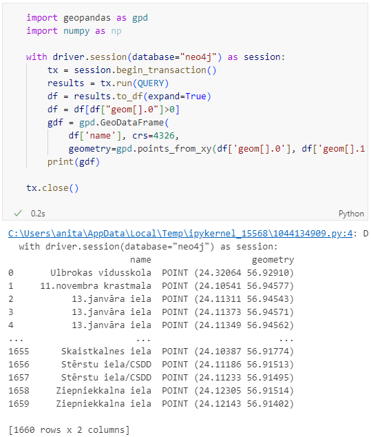
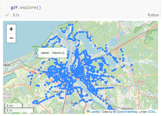
Nice. There we have our GTFS stops, their names and their locations. But how to put them on a map?
import geopandas as gpd
import numpy as np

with driver.session(database="neo4j") as session:
    tx = session.begin_transaction()
    results = tx.run(QUERY)
    df = results.to_df(expand=True)
    df = df[df["geom[].0"]>0]
    gdf = gpd.GeoDataFrame(
        df['name'], crs=4326,
        geometry=gpd.points_from_xy(df['geom[].0'], df['geom[].1']))
    print(gdf)

tx.close()
Since some of the nodes lack geometries, I added a quick and dirty hack to get rid of these nodes because — otherwise — gdf.explore() will complain about None geometries.
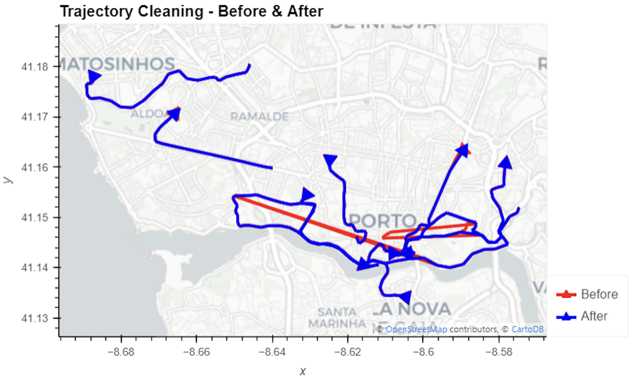
written together with my fellow co-authors and EMERALDS project team members Argyrios Kyrgiazos and Helen McKenzie.
In this blog post, we walk you through a trajectory hotspot analysis using open taxi trajectory data from Kaggle, combining data preparation with MovingPandas (including the new OutlierCleaner illustrated above) and spatiotemporal hotspot analysis from Carto.
In a recent post, we looked into a graph-based model for maritime mobility data and how it may be represented in Neo4J. Today, I want to look into another type of mobility data: public transport schedules in GTFS format.
Since a GTFS export is basically a ZIP archive full of CSVs, we will be making good use of Neo4Js CSV loading capabilities. The basic script for importing the stops file and creating point geometries from lat and lon values would be:
LOAD CSV with headers
FROM "file:///stops.txt"
AS row
CREATE (:Stop {
   stop_id: row["stop_id"],
   name: row["stop_name"],
   location: point({
    longitude: toFloat(row["stop_lon"]),
    latitude: toFloat(row["stop_lat"])
    })
})
This requires that the stops.txt is located in the import directory of your Neo4J database. When we run the above script and the file is missing, Neo4J will tell us where it tried to look for it. In my case, the directory ended up being:
So, let’s put all GTFS CSVs into that directory and we should be good to go.
Let’s start with the agency file:
load csv with headers from
'file:///agency.txt' as row
create (a:Agency {
   id: row.agency_id,
   name: row.agency_name,
   url: row.agency_url,
   timezone: row.agency_timezone,
   lang: row.agency_lang
});
… Added 1 label, created 1 node, set 5 properties, completed after 31 ms.
The routes file does not include agency info but, luckily, there is only one agency, so we can hard-code it:
load csv with headers from
'file:///routes.txt' as row
match (a:Agency {id: "rigassatiksme"})
create (a)-[:OPERATES]->(r:Route {
   id: row.route_id,
   shortName: row.route_short_name,
   longName: row.route_long_name,
   type: toInteger(row.route_type)
});
… Added 81 labels, created 81 nodes, set 324 properties, created 81 relationships, completed after 28 ms.
From stops, I’m removing non-existent or empty columns:
load csv with headers from
'file:///stops.txt' as row
create (s:Stop {
   id: row.stop_id,
   name: row.stop_name,
   location: point({
      latitude: toFloat(row.stop_lat),
      longitude: toFloat(row.stop_lon)
   }),
   code: row.stop_code
});
… Added 1671 labels, created 1671 nodes, set 5013 properties, completed after 71 ms.
From trips, I’m also removing non-existent or empty columns:
load csv with headers from
'file:///trips.txt' as row
match (r:Route {id: row.route_id})
create (r)<-[:USES]-(t:Trip {
   id: row.trip_id,
   serviceId: row.service_id,
   headSign: row.trip_headsign,
   direction_id: toInteger(row.direction_id),
   blockId: row.block_id,
   shapeId: row.shape_id
});
… Added 14427 labels, created 14427 nodes, set 86562 properties, created 14427 relationships, completed after 875 ms.
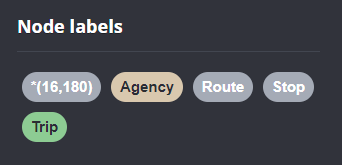
Slowly getting there. We now have around 16k nodes in our graph:
Finally, it’s stop times time. This is where the serious information is. This file is much larger than all previous ones with over 300k lines (i.e. times when an PT vehicle stops).
:auto
load csv with headers from
'file:///stop_times.txt' as row
CALL { with row
match (t:Trip {id: row.trip_id}), (s:Stop {id: row.stop_id})
create (t)<-[:BELONGS_TO]-(st:StopTime {
   arrivalTime: row.arrival_time,
   departureTime: row.departure_time,
   stopSequence: toInteger(row.stop_sequence)})-[:STOPS_AT]->(s)
} IN TRANSACTIONS OF 10 ROWS;
… Added 351388 labels, created 351388 nodes, set 1054164 properties, created 702776 relationships, completed after 1364220 ms.
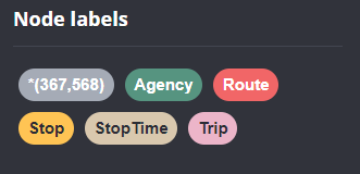
As you can see, this took a while. But now we have all nodes in place:
The final statement adds additional relationships between consecutive stop times:
call apoc.periodic.iterate('match (t:Trip) return t',
'match (t)<-[:BELONGS_TO]-(st) with st order by st.stopSequence asc
with collect(st) as stops
unwind range(0, size(stops)-2) as i
with stops[i] as curr, stops[i+1] as next
merge (curr)-[:NEXT_STOP]->(next)', {batchmode: "BATCH", parallel:true, parallel:true, batchSize:1});
This fails with: There is no procedure with the name apoc.periodic.iterate registered for this database instance. Please ensure you've spelled the procedure name correctly and that the procedure is properly deployed.
So, let’s install APOC. That’s a plugin which we can install into our database from within Neo4J Desktop:
After restarting the db, we can run the query:
No errors. Sounds good.
Let’s have a look at what we ended up with. Here are 25 random Trips. I expanded one of them to show its associated StopTimes. We can see the relations between consecutive StopTimes and I’ve expanded the final five StopTimes to show their linked Stops:
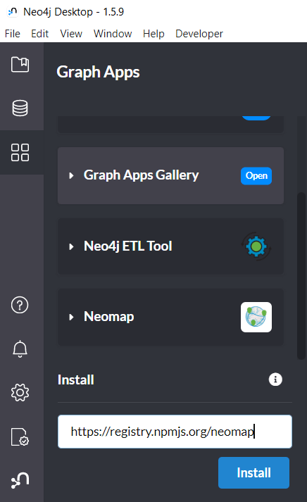
I also wanted to visualize the stops on a map. And there used to be a neat app called Neomap which can be installed easily:
This summer, I had the honor to — once again — speak at the OpenGeoHub Summer School. This time, I wanted to challenge the students and myself by not just doing MovingPandas but by introducing both MovingPandas and DVC for Mobility Data Science.
I’ve previously written about DVC and how it may be used to track geoprocessing workflows with QGIS & DVC. In my summer school session, we go into details on how to use DVC to keep track of MovingPandas movement data analytics workflow.
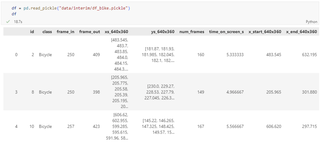
The bicycle trajectory coordinates are stored in two separate lists: xs_640x360 and ys640x360:
This format is kind of similar to the Kaggle Taxi dataset, we worked with in the previous post. However, to use the solution we implemented there, we need to combine the x and y coordinates into nice (x,y) tuples:
Afterwards, we can create the points and compute the proper timestamps from the frame numbers:
def compute_datetime(row):
    # some educated guessing going on here: the paper states that the video covers 2021-06-09 07:00-08:00
    d = datetime(2021,6,9,7,0,0) + (row['frame_in'] + row['running_number']) * timedelta(seconds=2)
    return d
def create_point(xy):
    try:
        return Point(xy)
    except TypeError:  # when there are nan values in the input data
        return None
new_df = df.head().explode('coordinates')
new_df['geometry'] = new_df['coordinates'].apply(create_point)
new_df['running_number'] = new_df.groupby('id').cumcount()
new_df['datetime'] = new_df.apply(compute_datetime, axis=1)
new_df.drop(columns=['coordinates', 'frame_in', 'running_number'], inplace=True)
new_df
Once the points and timestamps are ready, we can create the MovingPandas TrajectoryCollection. Note how we explicitly state that there is no CRS for this dataset (crs=None):
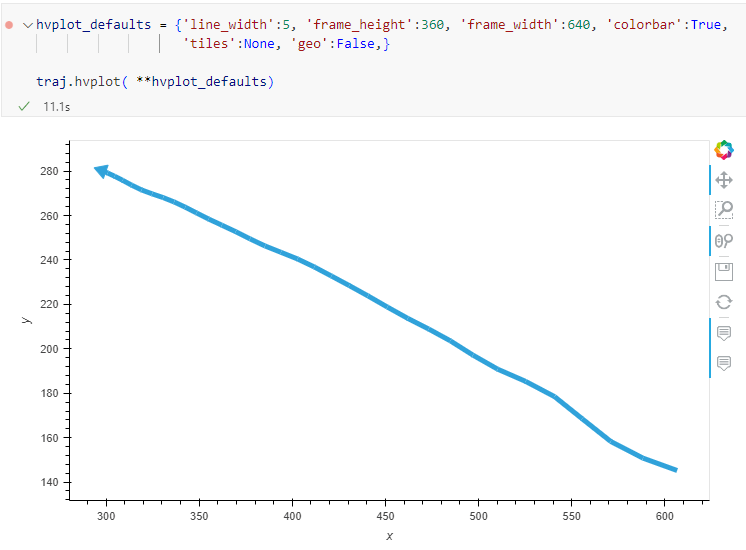
Similarly, to plot these trajectories, we should tell hvplot that it should not fetch any background map tiles (’tiles’:None) and that the coordinates are not geographic (‘geo’:False):
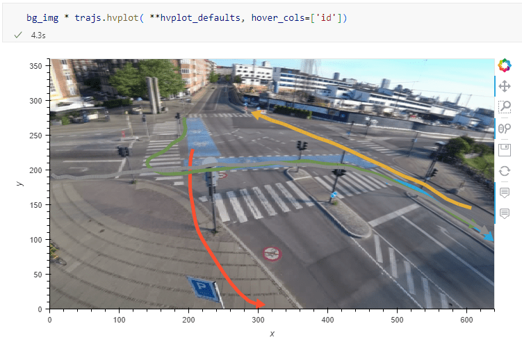
One important caveat is that speed will be calculated in pixels per second. So when we plot the bicycle speed, the segments closer to the camera will appear faster than the segments in the background:
To fix this issue, we would have to correct for the distortions of the camera lens and perspective. I’m sure that there is specialized software for this task but, for the purpose of this post, I’m going to grab the opportunity to finally test out the VectorBender plugin.
Georeferencing the trajectories using QGIS VectorBender plugin
Let’s load the five test trajectories and the camera image to QGIS. To make sure that they align properly, both are set to the same CRS and I’ve created the following basic world file for the camera image:
1
0
0
-1
0
360
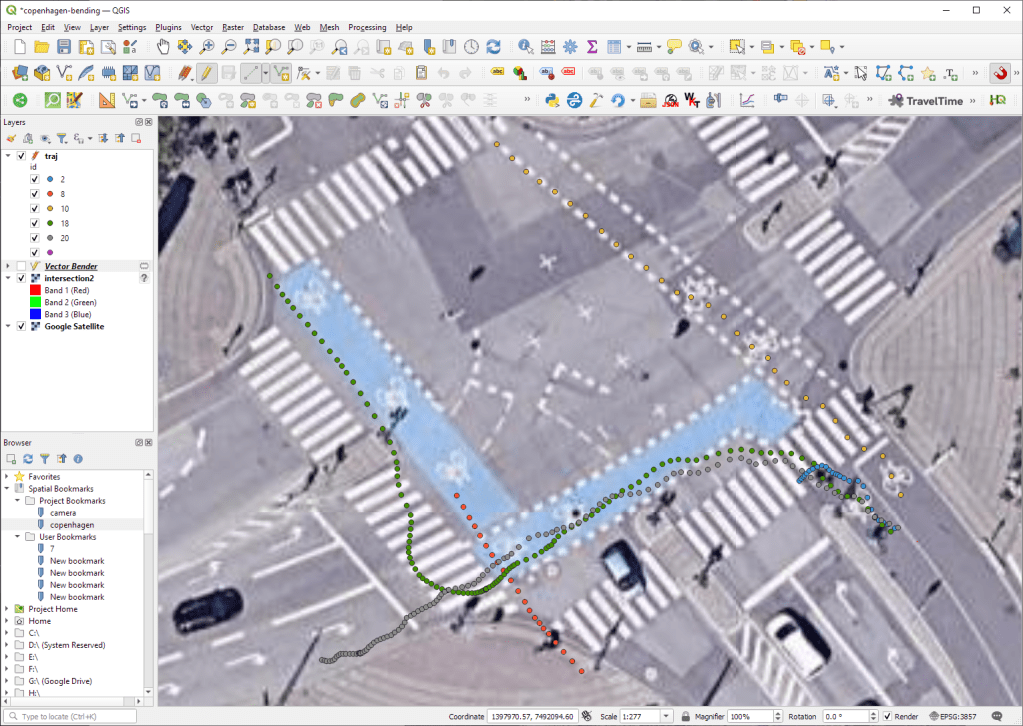
Then we can use the VectorBender tools to georeference the trajectories by linking locations from the camera image to locations on aerial images. You can see the whole process in action here:
After around 15 minutes linking control points, VectorBender comes up with the following georeferenced trajectory result:
Not bad for a quick-and-dirty hack. Some points on the borders of the image could not be georeferenced since I wasn’t always able to identify suitable control points at the camera image borders. So it won’t be perfect but should improve speed estimates.
In the previous post, we — creatively ;-) — used MobilityDB to visualize stationary IOT sensor measurements.
This post covers the more obvious use case of visualizing trajectories. Thus bringing together the MobilityDB trajectories created in Detecting close encounters using MobilityDB 1.0 and visualization using Temporal Controller.
Like in the previous post, the valueAtTimestamp function does the heavy lifting. This time, we also apply it to the geometry time series column called trip:
It’s been a while since we last talked about MobilityDB in 2019 and 2020. Since then, the project has come a long way. It joined OSGeo as a community project and formed a first PSC, including the project founders Mahmoud Sakr and Esteban Zimányi as well as Vicky Vergara (of pgRouting fame) and yours truly.
This post is a quick teaser tutorial from zero to computing closest points of approach (CPAs) between trajectories using MobilityDB.
Setting up MobilityDB with Docker
The easiest way to get started with MobilityDB is to use the ready-made Docker container provided by the project. I’m using Docker and WSL (Windows Subsystem Linux on Windows 10) here. Installing WLS/Docker is out of scope of this post. Please refer to the official documentation for your operating system.
Once Docker is ready, we can pull the official container and fire it up:
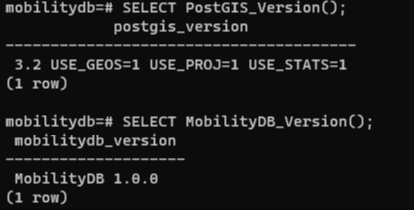
Currently, the container provides PostGIS 3.2 and MobilityDB 1.0:
Loading movement data into MobilityDB
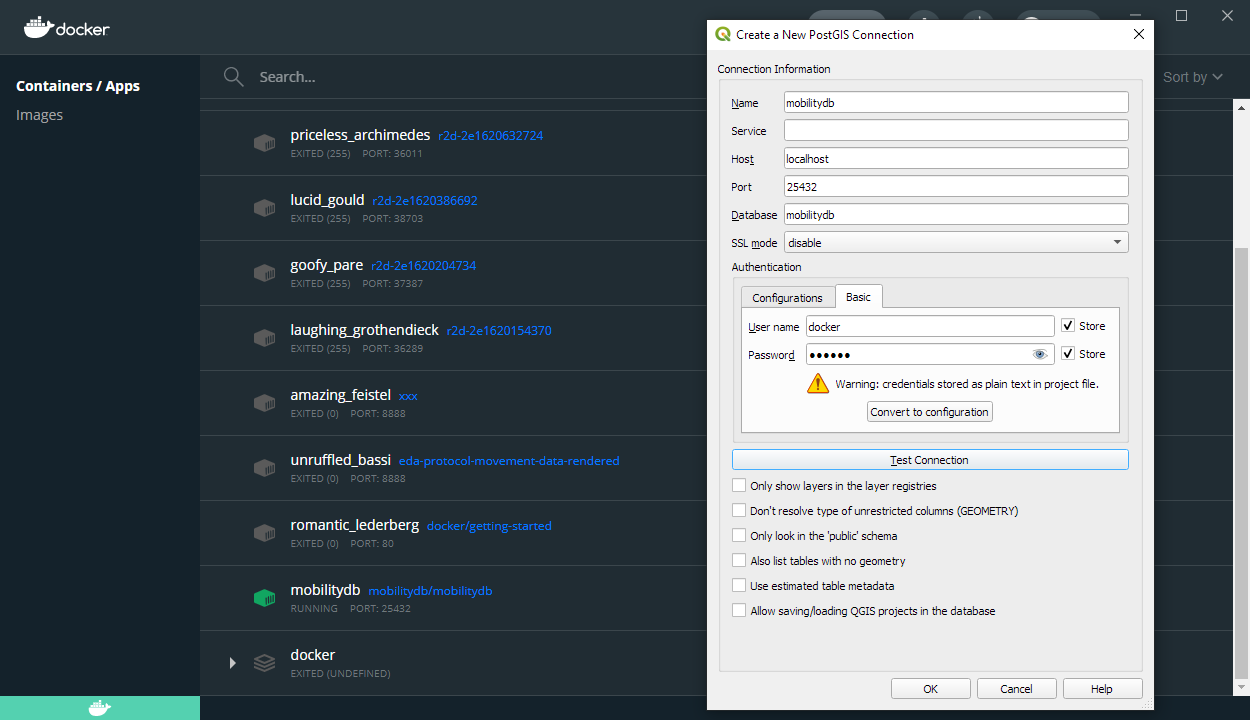
Once the container is running, we can already connect to it from QGIS. This is my preferred way to load data into MobilityDB because we can simply drag-and-drop any timestamped point layer into the database:
For this post, I’m using an AIS data sample in the region of Gothenburg, Sweden.
After loading this data into a new table called ais, it is necessary to remove duplicate and convert timestamps:
CREATE TABLE AISInputFiltered AS
SELECT DISTINCT ON("MMSI","Timestamp") *
FROM ais;

ALTER TABLE AISInputFiltered ADD COLUMN t timestamp;
UPDATE AISInputFiltered SET t = "Timestamp"::timestamp;
Afterwards, we can create the MobilityDB trajectories:
CREATE TABLE Ships AS
SELECT "MMSI" mmsi,
tgeompoint_seq(array_agg(tgeompoint_inst(Geom, t) ORDER BY t)) AS Trip,
tfloat_seq(array_agg(tfloat_inst("SOG", t) ORDER BY t) FILTER (WHERE "SOG" IS NOT NULL) ) AS SOG,
tfloat_seq(array_agg(tfloat_inst("COG", t) ORDER BY t) FILTER (WHERE "COG" IS NOT NULL) ) AS COG
FROM AISInputFiltered
GROUP BY "MMSI";

ALTER TABLE Ships ADD COLUMN Traj geometry;
UPDATE Ships SET Traj = trajectory(Trip);
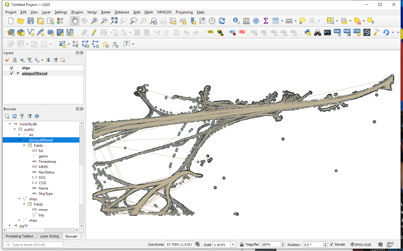
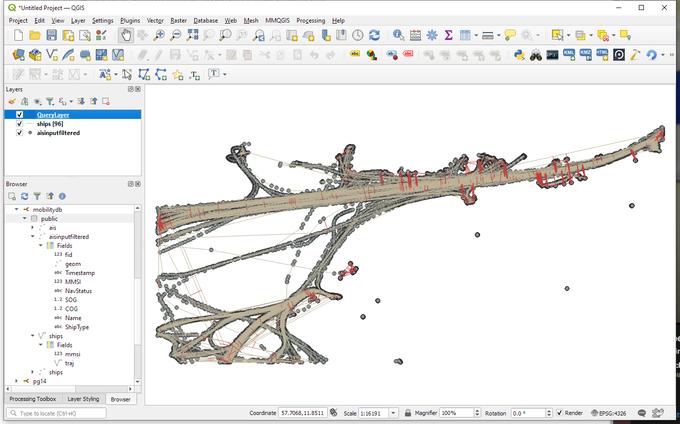
Once this is done, we can load the resulting Ships layer and the trajectories will be loaded as lines:
Computing closest points of approach
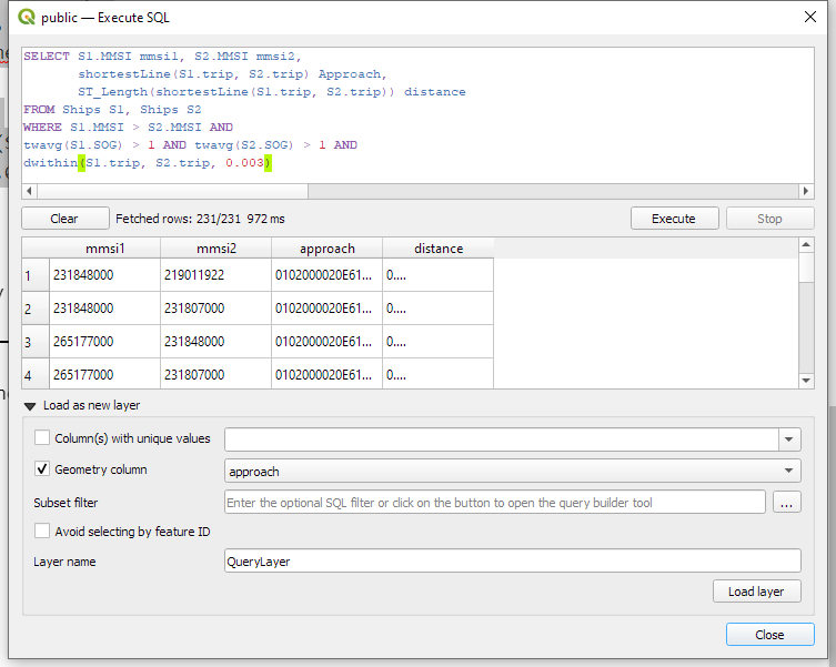
To compute the closest point of approach between two moving objects, MobilityDB provides a shortestLine function. To be correct, this function computes the line connecting the nearest approach point between the two tgeompoint_seq. In addition, we can use the time-weighted average function twavg to compute representative average movement speeds and eliminate stationary or very slowly moving objects:
SELECT S1.MMSI mmsi1, S2.MMSI mmsi2,
       shortestLine(S1.trip, S2.trip) Approach,
       ST_Length(shortestLine(S1.trip, S2.trip)) distance
FROM Ships S1, Ships S2
WHERE S1.MMSI > S2.MMSI AND
twavg(S1.SOG) > 1 AND twavg(S2.SOG) > 1 AND
dwithin(S1.trip, S2.trip, 0.003)
In the QGIS Browser panel, we can right-click the MobilityDB connection to bring up an SQL input using Execute SQL:
The resulting query layer shows where moving objects get close to each other:
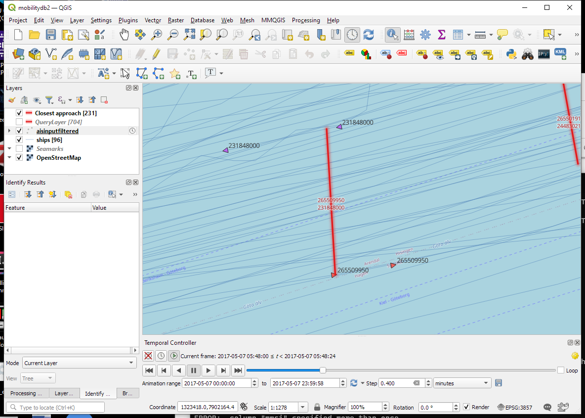
To better see what’s going on, we’ll look at individual CPAs:
Having a closer look with the Temporal Controller
Since our filtered AIS layer has proper timestamps, we can animate it using the Temporal Controller. This enables us to replay the movement and see what was going on in a certain time frame.
I let the animation run and stopped it once I spotted a close encounter. Looking at the AIS points and the shortest line, we can see that MobilityDB computed the CPAs along the trajectories:
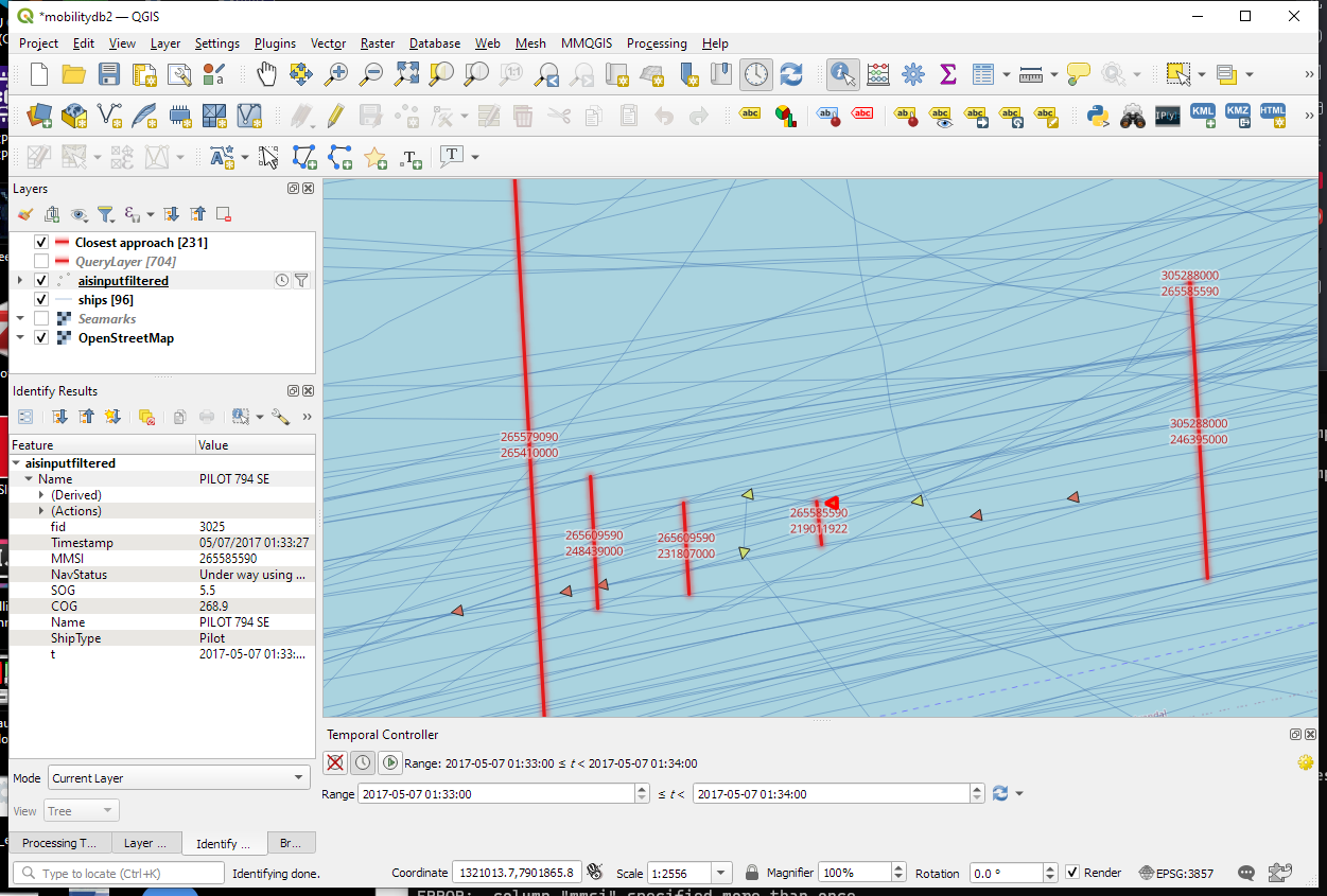
A more targeted way to investigate a specific CPA is to use the Temporal Controllers’ fixed temporal range mode to jump to a specific time frame. This is helpful if we already know the time frame we are interested in. For the CPA use case, this means that we can look up the timestamp of a nearby AIS position and set up the Temporal Controller accordingly:
More
I hope you enjoyed this quick dive into MobilityDB. For more details, including talks by the project founders, check out the project website.
First time, we talked about the OGC Moving Features standard in a post from 2017. Back then, we looked at the proposed standard way to encode trajectories in CSV and discussed its issues. Since then, the Moving Features working group at OGC has not been idle. Besides the CSV and XML encodings, they have designed a new JSON encoding that addresses many of the downsides of the previous two. You can read more about this in our 2020 preprint “From Simple Features to Moving Features and Beyond”.
Basically Moving Features JSON (MF-JSON) is heavily inspired by GeoJSON and it comes with a bunch of mandatory and optional key/value pairs. There is support for static properties as well as dynamic temporal properties and, of course, temporal geometries (yes geometries, not just points).
I think this format may have an actual chance of gaining more widespread adoption.
Inspired by Pandas.read_csv() and GeoPandas.read_file(), I’ve started implementing a read_mf_json() function in MovingPandas. So far, it supports basic MovingFeature JSONs with MovingPoint geometry:
You’ll need to use the current development version to test this feature.
Next steps will be MovingFeatureCollection JSONs and support for static as well as temporal properties. We’ll have to see if MovingPandas can be extended to go beyond moving point geometries. Storing moving linestrings and polygons in the GeoDataFrame will be the simple part but analytics and visualization will certainly be more tricky.