In a previous post, I showed how to use docker to run a single application (GeoServer) in a container and connect to it from your local QGIS install. Today’s post is about running a whole bunch of containers that interact with each other. More specifically, I’m using the images provided by Geodocker. The Geodocker repository provides a setup containing Accumulo, GeoMesa, and GeoServer. If you are not familiar with GeoMesa yet:

GeoMesa is an open-source, distributed, spatio-temporal database built on a number of distributed cloud data storage systems … GeoMesa aims to provide as much of the spatial querying and data manipulation to Accumulo as PostGIS does to Postgres.

The following sections show how to load data into GeoMesa, perform basic queries via command line, and finally publish data to GeoServer. The content is based largely on two GeoMesa tutorials: Geodocker: Bootstrapping GeoMesa Accumulo and Spark on AWS and Map-Reduce Ingest of GDELT, as well as Diethard Steiner’s post on Accumulo basics. The key difference is that this tutorial is written to be run locally (rather than on AWS or similar infrastructure) and that it spells out all user names and passwords preconfigured in Geodocker.

This guide was tested on Ubuntu and assumes that Docker is already installed. If you haven’t yet, you can install Docker as described in Install using the repository.

To get Geodocker set up, we need to get the code from Github and run the docker-compose command:

$ git clone https://github.com/geodocker/geodocker-geomesa.git
$ cd geodocker-geomesa/geodocker-accumulo-geomesa/
$ docker-compose up

This will take a while.

When docker-compose is finished, use a second console to check the status of all containers:

$ docker ps
CONTAINER ID        IMAGE                                     COMMAND                  CREATED             STATUS              PORTS                                        NAMES
4a238494e15f        quay.io/geomesa/accumulo-geomesa:latest   "/sbin/entrypoint...."   19 hours ago        Up 23 seconds                                                    geodockeraccumulogeomesa_accumulo-tserver_1
e2e0df3cae98        quay.io/geomesa/accumulo-geomesa:latest   "/sbin/entrypoint...."   19 hours ago        Up 22 seconds       0.0.0.0:50095-&gt;50095/tcp                     geodockeraccumulogeomesa_accumulo-monitor_1
e7056f552ef0        quay.io/geomesa/accumulo-geomesa:latest   "/sbin/entrypoint...."   19 hours ago        Up 24 seconds                                                    geodockeraccumulogeomesa_accumulo-master_1
dbc0ffa6c39c        quay.io/geomesa/hdfs:latest               "/sbin/entrypoint...."   19 hours ago        Up 23 seconds                                                    geodockeraccumulogeomesa_hdfs-data_1
20e90a847c5b        quay.io/geomesa/zookeeper:latest          "/sbin/entrypoint...."   19 hours ago        Up 24 seconds       2888/tcp, 0.0.0.0:2181-&gt;2181/tcp, 3888/tcp   geodockeraccumulogeomesa_zookeeper_1
997b0e5d6699        quay.io/geomesa/geoserver:latest          "/opt/tomcat/bin/c..."   19 hours ago        Up 22 seconds       0.0.0.0:9090-&gt;9090/tcp                       geodockeraccumulogeomesa_geoserver_1
c17e149cda50        quay.io/geomesa/hdfs:latest               "/sbin/entrypoint...."   19 hours ago        Up 23 seconds       0.0.0.0:50070-&gt;50070/tcp                     geodockeraccumulogeomesa_hdfs-name_1

At the time of writing this post, the Geomesa version installed in this way is 1.3.2:

$ docker exec geodockeraccumulogeomesa_accumulo-master_1 geomesa version
GeoMesa tools version: 1.3.2
Commit ID: 2b66489e3d1dbe9464a9860925cca745198c637c
Branch: 2b66489e3d1dbe9464a9860925cca745198c637c
Build date: 2017-07-21T19:56:41+0000

Loading data

First we need to get some data. The available tutorials often refer to data published by the GDELT project. Let’s download data for three days, unzip it and copy it to the geodockeraccumulogeomesa_accumulo-master_1 container for further processing:

$ wget http://data.gdeltproject.org/events/20170710.export.CSV.zip
$ wget http://data.gdeltproject.org/events/20170711.export.CSV.zip
$ wget http://data.gdeltproject.org/events/20170712.export.CSV.zip
$ unzip 20170710.export.CSV.zip
$ unzip 20170711.export.CSV.zip
$ unzip 20170712.export.CSV.zip
$ docker cp ~/Downloads/geomesa/gdelt/20170710.export.CSV geodockeraccumulogeomesa_accumulo-master_1:/tmp/20170710.export.CSV
$ docker cp ~/Downloads/geomesa/gdelt/20170711.export.CSV geodockeraccumulogeomesa_accumulo-master_1:/tmp/20170711.export.CSV
$ docker cp ~/Downloads/geomesa/gdelt/20170712.export.CSV geodockeraccumulogeomesa_accumulo-master_1:/tmp/20170712.export.CSV

Loading or importing data is called “ingesting” in Geomesa parlance. Since the format of GDELT data is already predefined (the CSV mapping is defined in geomesa-tools/conf/sfts/gdelt/reference.conf), we can ingest the data:

$ docker exec geodockeraccumulogeomesa_accumulo-master_1 geomesa ingest -c geomesa.gdelt -C gdelt -f gdelt -s gdelt -u root -p GisPwd /tmp/20170710.export.CSV
$ docker exec geodockeraccumulogeomesa_accumulo-master_1 geomesa ingest -c geomesa.gdelt -C gdelt -f gdelt -s gdelt -u root -p GisPwd /tmp/20170711.export.CSV
$ docker exec geodockeraccumulogeomesa_accumulo-master_1 geomesa ingest -c geomesa.gdelt -C gdelt -f gdelt -s gdelt -u root -p GisPwd /tmp/20170712.export.CSV

Once the data is ingested, we can have a look at the the created table by asking GeoMesa to describe the created schema:

$ docker exec geodockeraccumulogeomesa_accumulo-master_1 geomesa describe-schema -c geomesa.gdelt -f gdelt -u root -p GisPwd
INFO  Describing attributes of feature 'gdelt'
globalEventId       | String
eventCode           | String
eventBaseCode       | String
eventRootCode       | String
isRootEvent         | Integer
actor1Name          | String
actor1Code          | String
actor1CountryCode   | String
actor1GroupCode     | String
actor1EthnicCode    | String
actor1Religion1Code | String
actor1Religion2Code | String
actor2Name          | String
actor2Code          | String
actor2CountryCode   | String
actor2GroupCode     | String
actor2EthnicCode    | String
actor2Religion1Code | String
actor2Religion2Code | String
quadClass           | Integer
goldsteinScale      | Double
numMentions         | Integer
numSources          | Integer
numArticles         | Integer
avgTone             | Double
dtg                 | Date    (Spatio-temporally indexed)
geom                | Point   (Spatially indexed)

User data:
  geomesa.index.dtg     | dtg
  geomesa.indices       | z3:4:3,z2:3:3,records:2:3
  geomesa.table.sharing | false

In the background, our data is stored in Accumulo tables. For a closer look, open an interactive terminal in the Accumulo master image:

$ docker exec -i -t geodockeraccumulogeomesa_accumulo-master_1 /bin/bash

and open the Accumulo shell:

# accumulo shell -u root -p GisPwd

When we store data in GeoMesa, there is not only one table but several. Each table has a specific purpose: storing metadata, records, or indexes. All tables get prefixed with the catalog table name:

root@accumulo> tables
accumulo.metadata
accumulo.replication
accumulo.root
geomesa.gdelt
geomesa.gdelt_gdelt_records_v2
geomesa.gdelt_gdelt_z2_v3
geomesa.gdelt_gdelt_z3_v4
geomesa.gdelt_queries
geomesa.gdelt_stats

By default, GeoMesa creates three indices:
Z2: for queries with a spatial component but no temporal component.
Z3: for queries with both a spatial and temporal component.
Record: for queries by feature ID.

But let’s get back to GeoMesa …

Querying data

Now we are ready to query the data. Let’s perform a simple attribute query first. Make sure that you are in the interactive terminal in the Accumulo master image:

$ docker exec -i -t geodockeraccumulogeomesa_accumulo-master_1 /bin/bash

This query filters for a certain event id:

# geomesa export -c geomesa.gdelt -f gdelt -u root -p GisPwd -q "globalEventId='671867776'"
Using GEOMESA_ACCUMULO_HOME = /opt/geomesa
id,globalEventId:String,eventCode:String,eventBaseCode:String,eventRootCode:String,isRootEvent:Integer,actor1Name:String,actor1Code:String,actor1CountryCode:String,actor1GroupCode:String,actor1EthnicCode:String,actor1Religion1Code:String,actor1Religion2Code:String,actor2Name:String,actor2Code:String,actor2CountryCode:String,actor2GroupCode:String,actor2EthnicCode:String,actor2Religion1Code:String,actor2Religion2Code:String,quadClass:Integer,goldsteinScale:Double,numMentions:Integer,numSources:Integer,numArticles:Integer,avgTone:Double,dtg:Date,*geom:Point:srid=4326
d9e6ab555785827f4e5f03d6810bbf05,671867776,120,120,12,1,UNITED STATES,USA,USA,,,,,,,,,,,,3,-4.0,20,2,20,8.77192982456137,2007-07-13T00:00:00.000Z,POINT (-97 38)
INFO  Feature export complete to standard out in 2290ms for 1 features

If the attribute query runs successfully, we can advance to some geo goodness … that’s why we are interested in GeoMesa after all … and perform a spatial query:

# geomesa export -c geomesa.gdelt -f gdelt -u root -p GisPwd -q "CONTAINS(POLYGON ((0 0, 0 90, 90 90, 90 0, 0 0)),geom)" -m 3
Using GEOMESA_ACCUMULO_HOME = /opt/geomesa
id,globalEventId:String,eventCode:String,eventBaseCode:String,eventRootCode:String,isRootEvent:Integer,actor1Name:String,actor1Code:String,actor1CountryCode:String,actor1GroupCode:String,actor1EthnicCode:String,actor1Religion1Code:String,actor1Religion2Code:String,actor2Name:String,actor2Code:String,actor2CountryCode:String,actor2GroupCode:String,actor2EthnicCode:String,actor2Religion1Code:String,actor2Religion2Code:String,quadClass:Integer,goldsteinScale:Double,numMentions:Integer,numSources:Integer,numArticles:Integer,avgTone:Double,dtg:Date,*geom:Point:srid=4326
139346754923c07e4f6a3ee01a3f7d83,671713129,030,030,03,1,NIGERIA,NGA,NGA,,,,,LIBYA,LBY,LBY,,,,,1,4.0,16,2,16,-1.4060533085217,2017-07-10T00:00:00.000Z,POINT (5.43827 5.35886)
9e8e885e63116253956e40132c62c139,671928676,042,042,04,1,NIGERIA,NGA,NGA,,,,,OPEC,IGOBUSOPC,,OPC,,,,1,1.9,5,1,5,-0.90909090909091,2017-07-10T00:00:00.000Z,POINT (5.43827 5.35886)
d6c6162d83c72bc369f68bcb4b992e2d,671817380,043,043,04,0,OPEC,IGOBUSOPC,,OPC,,,,RUSSIA,RUS,RUS,,,,,1,2.8,2,1,2,-1.59453302961275,2017-07-09T00:00:00.000Z,POINT (5.43827 5.35886)
INFO  Feature export complete to standard out in 2127ms for 3 features

Functions that can be used in export command queries/filters are (E)CQL functions from geotools for the most part. More sophisticated queries require SparkSQL.

Publishing GeoMesa tables with GeoServer

To view data in GeoServer, go to http://localhost:9090/geoserver/web. Login with admin:geoserver.

First, we create a new workspace called “geomesa”.

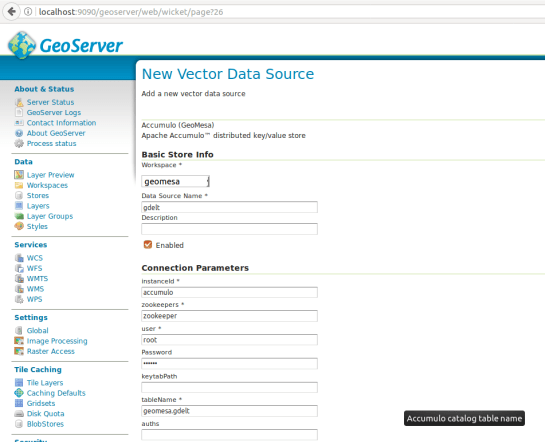
Then, we can create a new store of type Accumulo (GeoMesa) called “gdelt”. Use the following parameters:

instanceId = accumulo
zookeepers = zookeeper
user = root
password = GisPwd
tableName = geomesa.gdelt

Geodocker

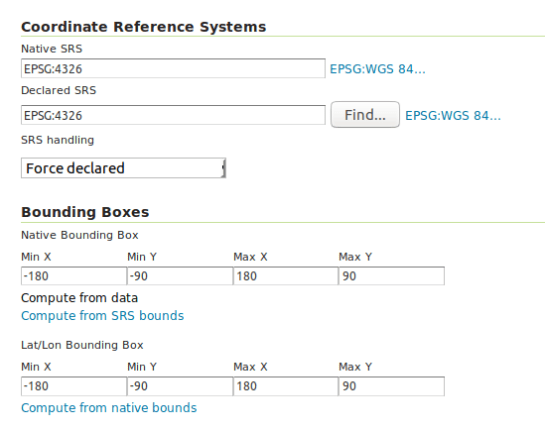
Then we can configure a Layer that publishes the content of our new data store. It is good to check the coordinate reference system settings and insert the bounding box information:

Geodocker2

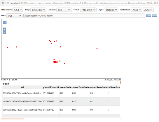
To preview the WMS, go to GeoServer’s preview:

http://localhost:9090/geoserver/geomesa/wms?service=WMS&version=1.1.0&request=GetMap&layers=geomesa:gdelt&styles=&bbox=-180.0,-90.0,180.0,90.0&width=768&height=384&srs=EPSG:4326&format=application/openlayers&TIME=2017-07-10T00:00:00.000Z/2017-07-10T01:00:00.000Z#

Which will look something like this:

GeoMesa data filtered using CQL in GeoServer preview

For more display options, check the official GeoMesa tutorial.

If you check the preview URL more closely, you will notice that it specifies a time window:

&TIME=2017-07-10T00:00:00.000Z/2017-07-10T01:00:00.000Z

This is exactly where QGIS TimeManager could come in: Using TimeManager for WMS-T layers. Interoperatbility for the win!

Movement data in GIS #7: animated trajectories with TimeManager

By underdark

2017-08-14

Movement data in GIS, QGIS, Visualization

19 Comments

In this post, we use TimeManager to visualize the position of a moving object over time along a trajectory. This is another example of what is possible thanks to QGIS’ geometry generator feature. The result can look like this:

What makes this approach interesting is that the trajectory is stored in PostGIS as a LinestringM instead of storing individual trajectory points. So there is only one line feature loaded in QGIS:

(In part 2 of this series, we already saw how a geometry generator can be used to visualize speed along a trajectory.)

The layer is added to TimeManager using t_start and t_end attributes to define the trajectory’s temporal extent.

TimeManager exposes an animation_datetime() function which returns the current animation timestamp, that is, the timestamp that is also displayed in the TimeManager dock, as well as on the map (if we don’t explicitly disable this option).

Once TimeManager is set up, we can edit the line style to add a point marker to visualize the position of the moving object at the current animation timestamp. To do that, we interpolate the position along the trajectory segments. The first geometry generator expression splits the trajectory in its segments:

The second geometry generator expression interpolates the position on the segment that contains the current TimeManager animation time:

The WHEN statement compares the trajectory segment’s start and end times to the current TimeManager animation time. Afterwards, the line_interpolate_point function is used to draw the point marker at the correct position along the segment:

CASE 
WHEN (
m(end_point(geometry_n($geometry,@geometry_part_num)))
> second(age(animation_datetime(),to_datetime('1970-01-01 00:00')))
AND
m(start_point(geometry_n($geometry,@geometry_part_num)))
<= second(age(animation_datetime(),to_datetime('1970-01-01 00:00')))
)
THEN
line_interpolate_point( 
  geometry_n($geometry,@geometry_part_num),
  1.0 * (
    second(age(animation_datetime(),to_datetime('1970-01-01 00:00')))
	- m(start_point(geometry_n($geometry,@geometry_part_num)))
  ) / (
    m(end_point(geometry_n($geometry,@geometry_part_num)))
	- m(start_point(geometry_n($geometry,@geometry_part_num)))
  ) 
  * length(geometry_n($geometry,@geometry_part_num))
)
END

Here is the animation result for a part of the trajectory between 08:00 and 09:00:

This post is part of a series. Read more about movement data in GIS.

Dynamic styling expressions with aggregates & variables

By underdark

2017-07-22

QGIS

In a recent post, we used aggregates for labeling purposes. This time, we will use them to create a dynamic data driven style, that is, a style that automatically adjusts to the minimum and maximum values of any numeric field … and that field will be specified in a variable!

But let’s look at this step by step. (This example uses climate.shp from the QGIS sample dataset.)

Here is a basic expression for data defined symbol color using a color ramp:

Similarly, we can configure a data defined symbol size to create a style like this:

Temperatures in July

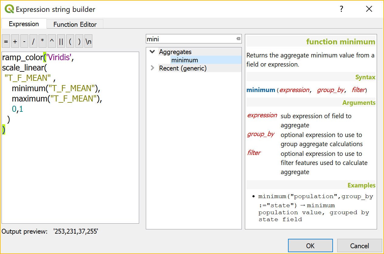
To stretch the color ramp from the attribute field’s minimum to maximum value, we can use aggregate functions:

That’s nice but if we want to be able to quickly switch to a different attribute field, we now have two expressions (one for color and one for size) to change. This can get repetitive and can be the source of errors if we miss an expression and don’t update it correctly …

To avoid these issues, we use a layer variable to store the name of the field that we want to use. Layer variables can be configured in layer properties:

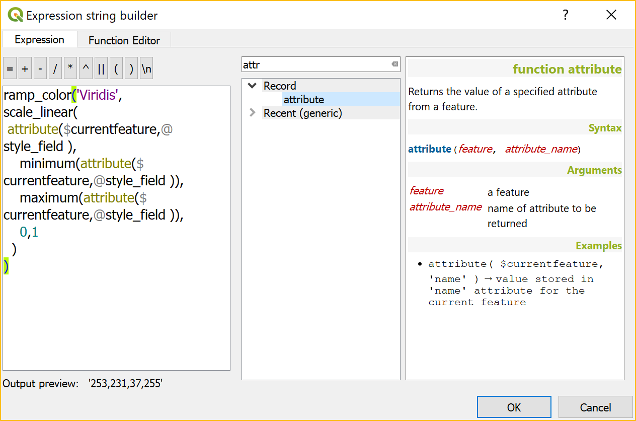
Then we adjust our expression to use the layer variable. Here is where it gets a bit tricky. We cannot simply replace the field name “T_F_JUL” with our new layer variable @style_field, since this creates an invalid expression. Instead, we have to use the attribute function:

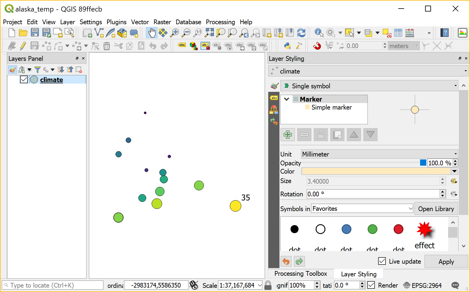
With this expression in place, we can now change the layer variable to T_M_JAN and the style automatically adjusts accordingly:

Temperatures in January

Note how the style also labels the point with the highest temperature? That’s because the style also defines an expression for the show labels option.

It is worth noting that, in most cases, temperature maps should not be styled using a color ramp that adjusts to a specific dataset’s min and max values. Instead, we would want a style with fixed value to color mapping that makes different datasets comparable. In many other use cases, however, it is very convenient to have a style that can automatically adapt to the data.

Docker basics with Geodocker GeoServer

By underdark

2017-07-12

GeoServer, GIS

5 Comments

Today’s post is mostly notes-to-self about using Docker. These steps were tested on a fresh Ubuntu 17.04 install.

Install Docker as described in https://docs.docker.com/engine/installation/linux/docker-ce/ubuntu/ “Install using the repository” section.

Then add the current user to the docker user group (otherwise, all docker commands have to be prefixed with sudo)

$ sudo gpasswd -a $USER docker
$ newgrp docker

Test run the hello world image

$ docker run hello-world

For some more Docker basics, see https://github.com/docker/labs/blob/master/beginner/chapters/alpine.md.

Pull Geodocker images, for example from https://quay.io/organization/geodocker

$ docker pull quay.io/geodocker/base
$ docker pull quay.io/geodocker/geoserver

Get a list of pulled images

$ docker images
REPOSITORY TAG IMAGE ID CREATED SIZE
quay.io/geodocker/geoserver latest c60753e05956 8 months ago 904MB
quay.io/geodocker/base latest 293209905a47 8 months ago 646MB

Test run quay.io/geodocker/base

$ docker run -it --rm quay.io/geodocker/base:latest java -version
java version "1.8.0_45"
Java(TM) SE Runtime Environment (build 1.8.0_45-b14)
Java HotSpot(TM) 64-Bit Server VM (build 25.45-b02, mixed mode)

Run quay.io/geodocker/geoserver

$ docker run --name geoserver -e AUTHOR="Anita" \
 -d -P quay.io/geodocker/geoserver

The important options are:

-d … Run container in background and print container ID

-P … Publish all exposed ports to random ports

Check if the image is running

$ docker ps
CONTAINER ID IMAGE COMMAND CREATED STATUS PORTS NAMES
684598b57868 quay.io/geodocker/geoserver "/opt/tomcat/bin/c..." 
2 hours ago Up 2 hours 0.0.0.0:32772->9090/tcp geoserver

You can also check which ports to access using

$ docker port geoserver
9090/tcp -> 0.0.0.0:32772

Geoserver should now run on http://localhost:32772/geoserver/ (user=admin, password=geoserver)

For more tests, let’s connect to Geoserver from QGIS

All default example layers are listed

and can be loaded into QGIS

Even more aggregations: QGIS point cluster renderer

By underdark

2017-06-13

QGIS, Visualization

10 Comments

In the previous post, I demonstrated the aggregation support in QGIS expressions. Another popular request is to aggregate or cluster point features that are close to each other. If you have been following the QGIS project on mailing list or social media, you probably remember the successful cluster renderer crowd-funding campaign by North Road.

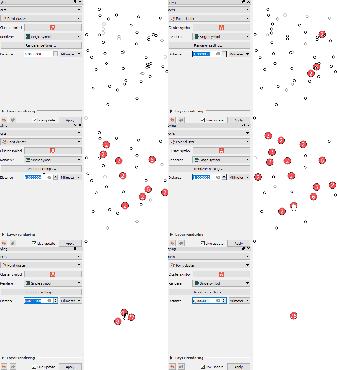
The point cluster renderer is implemented and can be tested in the current developer version. The renderer is highly customizable, for example, by styling the cluster symbol and adjusting the distance between points that should be in the same cluster:

Beyond this basic use case, the point cluster renderer can also be combined with categorized visualizations and clusters symbols can be colored in the corresponding category color and scaled by cluster size, as demoed in this video by the developer Nyall Dawson:

Aggregate all the things! (QGIS expression edition)

By underdark

2017-06-08

QGIS

12 Comments

In the past, aggregating field values was reserved to databases, virtual layers, or dedicated plugins, but since QGIS 2.16, there is a way to compute aggregates directly in QGIS expressions. This means that we can compute sums, means, counts, minimum and maximum values and more!

Here’s a quick tutorial to get you started:

Load the airports from the QGIS sample dataset. We’ll use the elevation values in the ELEV field for the following examples:

QGIS sample airport dataset – categorized by USE attribute

The most straightforward expressions are those that only have one parameter: the name of the field that should be aggregated, for example:

mean(ELEV)

We can also add a second parameter: a group-by field, for example, to group by the airport usage type, we use:

mean(ELEV,USE)

To top it all off, we can add a third parameter: a filter expression, for example, to show only military airports, we use:

mean(ELEV,USE,USE='Military')

Last but not least, all this aggregating goodness also works across layers! For example, here is the Alaska layer labeled with the airport layer feature count:

aggregate('airports','count',"ID")

If you are using relations, you can even go one step further and calculate aggregates on feature relations.

Upcoming QGIS3 features – exploring the current developer version

By underdark

2017-05-23

QGIS

5 Comments

There are tons of things going on under the hood of QGIS for the move from version 2 to version 3. Besides other things, we’ll have access to new versions of Qt and Python. If you are using a HiDPI screen, you should see some notable improvements in the user interface of QGIS 3.

But of course QGIS 3 is not “just” a move to updated dependencies. Like in any other release, there are many new features that we are looking forward to. This list is only a start, including tools that already landed in the developer version 2.99:

Improved geometry editing

When editing geometries, the node tool now behaves more like editing tools in webmaps: instead of double-clicking to add a new node, the tool automatically suggests a new node when the cursor hovers over a line segment.

In addition, improvements include an undo and redo panel for quick access to previous versions.

Improved Processing dialogs

Like many other parts of the QGIS user interface, Processing dialogs now prominently display the function help.

In addition, GDAL/OGR tools also show the underlying GDAL/OGR command which can be copy-pasted to use it somewhere else.

New symbols and predefined symbol groups

The default symbols have been reworked and categorized into different symbol groups. Of course, everything can be customized in the Symbol Library.

Search in layer and project properties

Both the layer properties and the project properties dialog now feature a search field in the top left corner. This nifty little addition makes it much easier to find specific settings fast.

Save images at custom sizes

Last but not least, a long awaited feature: It’s finally possible to specify the exact size and properties of images created using Project | Save as image.

Of course, we still expect many other features to arrive in 3.0. For example, one of the successful QGIS grant applications was for adding 3D support to QGIS. Additionally, there is an ongoing campaign to fund better layout and reporting functionality in QGIS print composer. Please support it if you can!

Movement data in GIS #6: updates from AGILE2017

By underdark

2017-05-21

GIS, Movement data in GIS

AGILE 2017 is the annual international conference on Geographic Information Science of the Association of Geographic Information Laboratories in Europe (AGILE) which was established in 1998 to promote academic teaching and research on GIS.

This years conference in Wageningen was my time at AGILE. I had the honor to present our recent work on pedestrian navigation with landmarks [Graser, 2017].

If you are interested in trying it, there is an online demo. The conference also provided numerous pointers toward ideas for future improvements, including [Götze and Boye, 2016] and [Du et al., 2017]

https://twitter.com/underdarkGIS/status/861917265217937409

On the issue of movement data in GIS, there weren’t too many talks on this topic at AGILE but on the conceptual side, I really enjoyed David Jonietz’ talk on how to describe trajectory processing steps:

Source: [Jonietz and Bucher, 2017]

In the pre-conference workshop I attended, there was also an interesting presentation on analyzing trajectory data with PostGIS by Phd candidate Meihan Jin.

https://twitter.com/underdarkGIS/status/861946078542925826

I’m also looking forward to reading [Wiratma et al., 2017] “On Measures for Groups of Trajectories” because I think that the presentation only scratched the surface.

References

[Du et al, 2017] Du, S., Wang, X., Feng, C. C., & Zhang, X. (2017). Classifying natural-language spatial relation terms with random forest algorithm. International Journal of Geographical Information Science, 31(3), 542-568.
[Götze and Boye, 2016] Götze, J., & Boye, J. (2016). Learning landmark salience models from users’ route instructions. Journal of Location Based Services, 10(1), 47-63.
[Graser, 2017] Graser, A. (2017). Towards landmark-based instructions for pedestrian navigation systems using OpenStreetMap, AGILE2017, Wageningen, Netherlands.
[Jonietz and Bucher, 2017] Jonietz, D., Bucher, D. (2017). Towards an Analytical Framework for Enriching Movement Trajectories with Spatio-Temporal Context Data, AGILE2017, Wageningen, Netherlands.
[Wiratma et al., 2017] Wiratma L., van Kreveld M., Löffler M. (2017) On Measures for Groups of Trajectories. In: Bregt A., Sarjakoski T., van Lammeren R., Rip F. (eds) Societal Geo-innovation. GIScience 2017. Lecture Notes in Geoinformation and Cartography. Springer, Cham

This post is part of a series. Read more about movement data in GIS.

Report from the Essen dev meeting

By underdark

2017-05-06

QGIS

3 Comments

From 28th April to 1st May the QGIS project organized another successful developer meeting at the Linuxhotel in Essen, Germany. Here is a quick summary of the key topics I’ve been working on during these days.

New logo rollout

It’s time to get the QGIS 3 logo out there! We’ve started changing our social media profile pictures and Website headers to the new design:

Resource sharing platform

In QGIS 3, the resource sharing platform will be available by default – just like the plugin manager is today in QGIS 2. We are constantly looking for people to share their mapping resources with the community. During this developer meeting Paolo Cavallini and I added two more SVG collections:

Road sign SVGs by Bertrand Bouteilles & Roulex_45 (CC BY-SA 3.0)

SVGs by Yury Ryabov & Pavel Sergeev (CC-BY 3.0)

Unified Add Layer button

We also discussed the unified add layer dialog and are optimistic that it will make its way into 3.0. The required effort for a first version is currently being estimated by the developers at Boundless.

Unified add layer button session

Draft dialog up for discussion

TimeManager

The new TimeManager version 2.4 fixes a couple of issues related to window resizing and display on HiDPI screens. Additionally, it now saves all label settings in the project file. This is the change log:

- Fixed #222: hide label if TimeManager is turned off
- Fixed #156: copy parent style to interpolation layer
- Fixed #109: save label settings in project
- Fixed window resizing issues in label options gui
- Fixed window resizing issues in video export gui
- Fixed HiDPI issues with arch gui