This summer, I had the honor to — once again — speak at the OpenGeoHub Summer School. This time, I wanted to challenge the students and myself by not just doing MovingPandas but by introducing both MovingPandas and DVC for Mobility Data Science.
I’ve previously written about DVC and how it may be used to track geoprocessing workflows with QGIS & DVC. In my summer school session, we go into details on how to use DVC to keep track of MovingPandas movement data analytics workflow.
written together with my fellow “Geocomputation with Python” co-authors Robin Lovelace, Michael Dorman, and Jakub Nowosad.
In this blog post, we talk about our experience teaching R and Python for geocomputation. The context of this blog post is the OpenGeoHub Summer School 2023 which has courses on R, Python and Julia. The focus of the blog post is on geographic vector data, meaning points, lines, polygons (and their ‘multi’ variants) and the attributes associated with them. We plan to cover raster data in a future post.
Since I’ve been on Twitter since 2011, this means that some media files are now lost. While the loss of a few low-res images is probably not a major loss for humanity, I would prefer to have some control over when and how content I created vanishes. So, to avoid losing more content, I have followed Jeff’s recommendation to create a proper archival page:
It is based on an export I pulled in October 2022 when I started to use Mastodon as my primary social media account. Unfortunately, this export did not include media files.
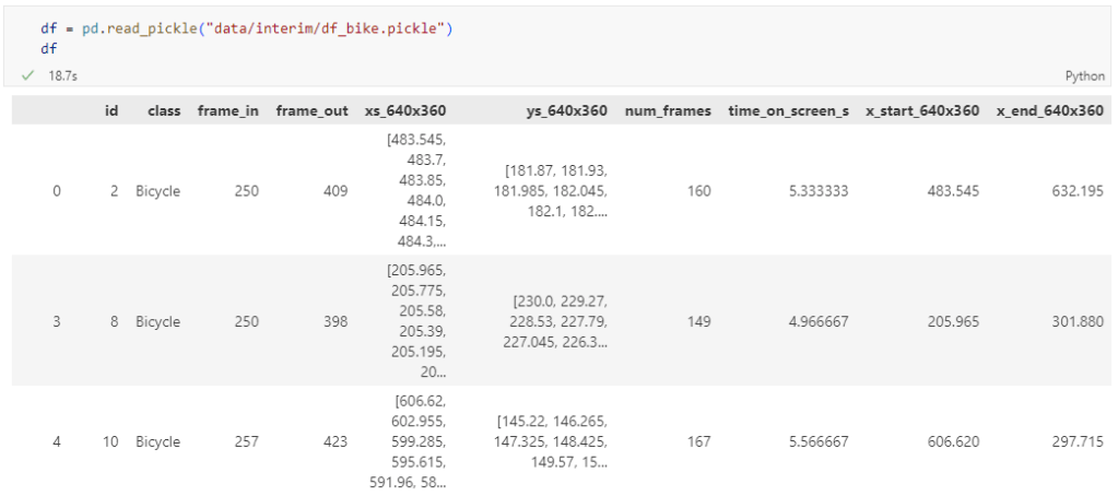
The bicycle trajectory coordinates are stored in two separate lists: xs_640x360 and ys640x360:
This format is kind of similar to the Kaggle Taxi dataset, we worked with in the previous post. However, to use the solution we implemented there, we need to combine the x and y coordinates into nice (x,y) tuples:
Afterwards, we can create the points and compute the proper timestamps from the frame numbers:
def compute_datetime(row):
    # some educated guessing going on here: the paper states that the video covers 2021-06-09 07:00-08:00
    d = datetime(2021,6,9,7,0,0) + (row['frame_in'] + row['running_number']) * timedelta(seconds=2)
    return d
def create_point(xy):
    try:
        return Point(xy)
    except TypeError:  # when there are nan values in the input data
        return None
new_df = df.head().explode('coordinates')
new_df['geometry'] = new_df['coordinates'].apply(create_point)
new_df['running_number'] = new_df.groupby('id').cumcount()
new_df['datetime'] = new_df.apply(compute_datetime, axis=1)
new_df.drop(columns=['coordinates', 'frame_in', 'running_number'], inplace=True)
new_df
Once the points and timestamps are ready, we can create the MovingPandas TrajectoryCollection. Note how we explicitly state that there is no CRS for this dataset (crs=None):
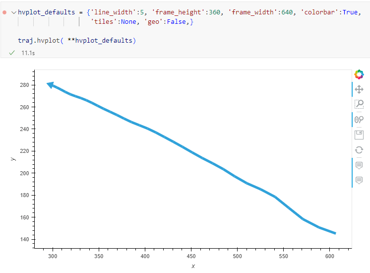
Similarly, to plot these trajectories, we should tell hvplot that it should not fetch any background map tiles (’tiles’:None) and that the coordinates are not geographic (‘geo’:False):
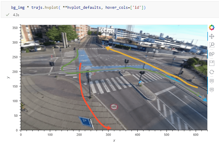
One important caveat is that speed will be calculated in pixels per second. So when we plot the bicycle speed, the segments closer to the camera will appear faster than the segments in the background:
To fix this issue, we would have to correct for the distortions of the camera lens and perspective. I’m sure that there is specialized software for this task but, for the purpose of this post, I’m going to grab the opportunity to finally test out the VectorBender plugin.
Georeferencing the trajectories using QGIS VectorBender plugin
Let’s load the five test trajectories and the camera image to QGIS. To make sure that they align properly, both are set to the same CRS and I’ve created the following basic world file for the camera image:
1
0
0
-1
0
360
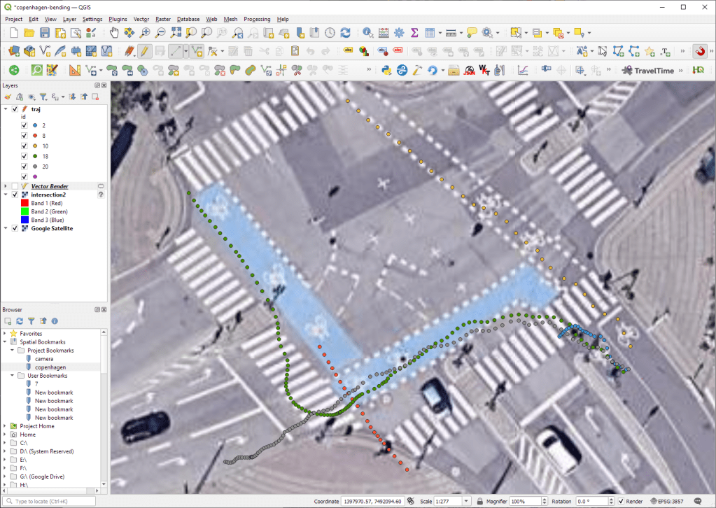
Then we can use the VectorBender tools to georeference the trajectories by linking locations from the camera image to locations on aerial images. You can see the whole process in action here:
After around 15 minutes linking control points, VectorBender comes up with the following georeferenced trajectory result:
Not bad for a quick-and-dirty hack. Some points on the borders of the image could not be georeferenced since I wasn’t always able to identify suitable control points at the camera image borders. So it won’t be perfect but should improve speed estimates.
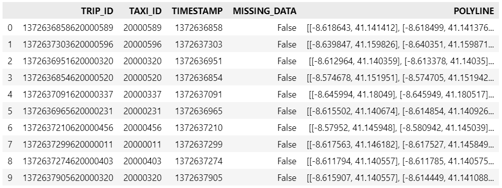
Kaggle’s “Taxi Trajectory Data from ECML/PKDD 15: Taxi Trip Time Prediction (II) Competition” is one of the most used mobility / vehicle trajectory datasets in computer science. However, in contrast to other similar datasets, Kaggle’s taxi trajectories are provided in a format that is not readily usable in MovingPandas since the spatiotemporal information is provided as:
TIMESTAMP: (integer) Unix Timestamp (in seconds). It identifies the trip’s start;
POLYLINE: (String): It contains a list of GPS coordinates (i.e. WGS84 format) mapped as a string. The beginning and the end of the string are identified with brackets (i.e. [ and ], respectively). Each pair of coordinates is also identified by the same brackets as [LONGITUDE, LATITUDE]. This list contains one pair of coordinates for each 15 seconds of trip. The last list item corresponds to the trip’s destination while the first one represents its start;
Therefore, we need to create a DataFrame with one point + timestamp per row before we can use MovingPandas to create Trajectories and analyze them.
But first things first. Let’s download the dataset:
import datetime
import pandas as pd
import geopandas as gpd
import movingpandas as mpd
import opendatasets as od
from os.path import exists
from shapely.geometry import Point

input_file_path = 'taxi-trajectory/train.csv'

def get_porto_taxi_from_kaggle():
    if not exists(input_file_path):
        od.download("https://www.kaggle.com/datasets/crailtap/taxi-trajectory")

get_porto_taxi_from_kaggle()
df = pd.read_csv(input_file_path, nrows=10, usecols=['TRIP_ID', 'TAXI_ID', 'TIMESTAMP', 'MISSING_DATA', 'POLYLINE'])
df.POLYLINE = df.POLYLINE.apply(eval)  # string to list
df
And now for the remodelling:
def unixtime_to_datetime(unix_time):
    return datetime.datetime.fromtimestamp(unix_time)

def compute_datetime(row):
    unix_time = row['TIMESTAMP']
    offset = row['running_number'] * datetime.timedelta(seconds=15)
    return unixtime_to_datetime(unix_time) + offset

def create_point(xy):
    try:
        return Point(xy)
    except TypeError:  # when there are nan values in the input data
        return None

new_df = df.explode('POLYLINE')
new_df['geometry'] = new_df['POLYLINE'].apply(create_point)
new_df['running_number'] = new_df.groupby('TRIP_ID').cumcount()
new_df['datetime'] = new_df.apply(compute_datetime, axis=1)
new_df.drop(columns=['POLYLINE', 'TIMESTAMP', 'running_number'], inplace=True)
new_df
And that’s it. Now we can create the trajectories:
That’s it. Now our MovingPandas.TrajectoryCollection is ready for further analysis.
By the way, the plot above illustrates a new feature in the recent MovingPandas 0.16 release which, among other features, introduced plots with arrow markers that show the movement direction. Other new features include a completely new custom distance, speed, and acceleration unit support. This means that, for example, instead of always getting speed in meters per second, you can now specify your desired output units, including km/h, mph, or nm/h (knots).
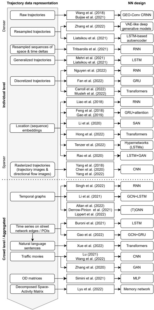
I’ve previously written about Movement data in GIS and the AI hype and today’s post is a follow-up in which I want to share with you a new review of the state of the art in deep learning from trajectory data.
Our review covers 8 use cases:
Location classification
Arrival time prediction
Traffic flow / activity prediction
Trajectory prediction
Trajectory classification
Next location prediction
Anomaly detection
Synthetic data generation
We particularly looked into the trajectory data preprocessing steps and the specific movement data representation used as input to train the neutral networks:
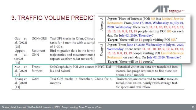
On a completely subjective note: the price for most surprising approach goes to natural language processing (NLP) Transfomers for traffic volume prediction.
The paper was presented at BMDA2023 and you can watch the full talk recording here:
DVC tracks data, parameters, and code. If anything changes, we simply rerun the process and DVC will figure out which stages need to be recomputed and which can be skipped by re-using cached results.
This can lead to huge time savings compared to re-running the whole model
I’m using DVC with the DVC plugin for VSCode but DVC can be used completely from the command line, if you prefer this appraoch.
Basically, what follows is a proof of concept: converting a QGIS Processing model to a DVC workflow. In the following screenshot, you can see the main stages
The QGIS model in the upper left corner
The Python script exported from the QGIS model builder in the lower left corner
The DVC stages in my dvc.yaml file in the upper right corner (And please ignore the hello world stage. It’s a left over from my first experiment)
The DVC DAG visualizing the sequence of stages. Looks similar to the QGIS model, doesn’t it ;-)
Besides the stage definitions in dvc.yaml, there’s a parameters file:
random-points:
  n: 10
buffer-points:
  size: 0.5
And, of course, the two stages, each as it’s own Python script.
First, random-points.py which reads the random-points.n parameter to create the desired number of points within the polygon defined in qgis3/data/test.geojson:
With these things in place, we can use dvc to run the workflow, either from within VSCode or from the command line. Here, you can see the workflow (and how dvc skips stages and fetches results from cache) in action:
If you try it out yourself, let me know what you think.
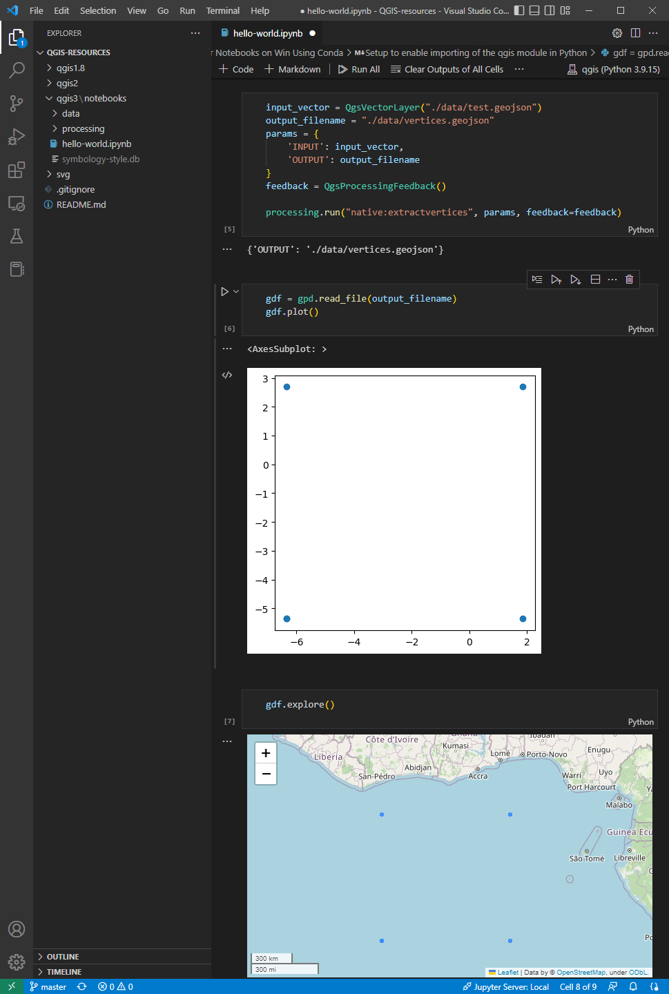
Similarly, we’ve seen posts on using PyQGIS in Jupyter notebooks. However, I find the setup with *.bat files rather tricky.
This post presents a way to set up a conda environment with QGIS that is ready to be used in Jupyter notebooks.
The first steps are to create a new environment and install QGIS. I use mamba for the installation step because it is faster than conda but you can use conda as well:
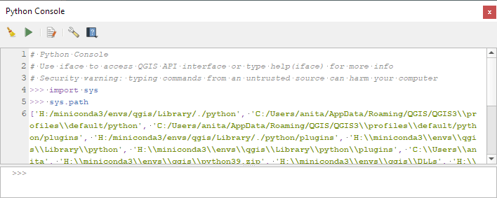
If we now try to import the qgis module in Python, we get an error:
(qgis) PS C:\Users\anita> python
Python 3.9.15 | packaged by conda-forge | (main, Nov 22 2022, 08:41:22) [MSC v.1929 64 bit (AMD64)] on win32
Type "help", "copyright", "credits" or "license" for more information.
>>> import qgis
Traceback (most recent call last):
  File "<stdin>", line 1, in <module>
ModuleNotFoundError: No module named 'qgis'
To fix this error, we need to get the paths from the Python console inside QGIS:
These releases are a huge step forward towards making MovingPandas easier to install with fewer mandatory dependencies. All interactive plotting libraries are now optional. So if you are using MovingPandas for trajectory data processing in the background and don’t need the interactive visualization features, the number of necessary libraries is now much lower. This (and the fact that GeoPandas is now shipped with OSGeo4W) will also make it easier to use MovingPandas in QGIS plugins.
In the previous post, we — creatively ;-) — used MobilityDB to visualize stationary IOT sensor measurements.
This post covers the more obvious use case of visualizing trajectories. Thus bringing together the MobilityDB trajectories created in Detecting close encounters using MobilityDB 1.0 and visualization using Temporal Controller.
Like in the previous post, the valueAtTimestamp function does the heavy lifting. This time, we also apply it to the geometry time series column called trip: