Last time, I wrote about the little details that make a good flow map. The data in that post was made up and simpler than your typical flow map. That’s why I wanted to redo it with real-world data. In this post, I’m using domestic migration data of Austria.

Raw migration data, line width scaled to flow strength

With 9 states, that makes 72 potential flow arrows. Since that’s too much to map, I’ve decided in a first step to only show flows with more than 1,000 people.

Following the recommendations mentioned in the previous post, I first designed a basic flow map where each flow direction is rendered as a black arrow:

Basic flow map

Even with this very limited number of flows, the map gets pretty crowded, particularly around the north-eastern node, the Austrian capital Vienna.

To reduce the number of incoming and outgoing lines at each node, I therefore decided to change to colored one-sided arrows that share a common geometry:

Colored one-sided arrows

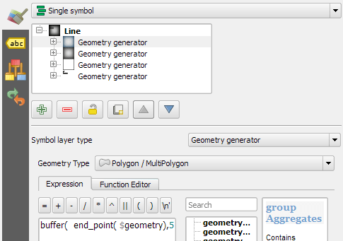
The arrow color is determined automatically based on the arrow direction using the following expression:

CASE WHEN
 "weight" < 1000 THEN color_rgba( 0,0,0,0)
WHEN
 x(start_point( $geometry)) - x(end_point($geometry)) < 0
THEN
 '#1f78b4'
ELSE
 '#ff7f00'
END

The same approach is used to control the side of the one-sided arrow head. The arrow symbol layer has two “arrow type” options for rendering the arrow head: on the inside of the curve or on the outside. This means that, if we wouldn’t use a data-defined approach, the arrow head would be on the same side – independent of the line geometry direction.

CASE WHEN
 x(start_point( $geometry)) - x(end_point($geometry)) < 0
THEN
 1
ELSE
 2
END

Obviously, this ignores the corner case of start and end points at the same x coordinate but, if necessary, this case can be added easily.

Of course the results are far from perfect and this approach still requires manual tweaking of the arrow geometries. Nonetheless, I think it’s very interesting to see how far we can push the limits of data-driven styling for flow maps.

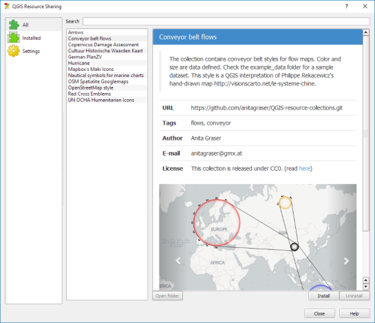
Give it a try! You’ll find the symbol and accompanying sample data on the QGIS resource sharing plugin platform:

Details of good flow maps

By underdark

2016-12-18

QGIS

42 Comments

In my previous post, I shared a flow map style that was inspired by a hand drawn map. Today’s post is inspired by a recent academic paper recommended to me by Radoslaw Panczak @RPanczak and Thomas Gratier @ThomasG77:

Jenny, B., Stephen, D. M., Muehlenhaus, I., Marston, B. E., Sharma, R., Zhang, E., & Jenny, H. (2016). Design principles for origin-destination flow maps. Cartography and Geographic Information Science, 1-15.

Jenny et al. (2016) performed a study on how to best design flow maps. The resulting design principles are:

number of flow overlaps should be minimized;

sharp bends and excessively asymmetric flows should be avoided;

acute intersection angles should be avoided;

flows must not pass under unconnected nodes;

flows should be radially arranged around nodes;

quantity is best represented by scaled flow width;

flow direction is best indicated with arrowheads;

arrowheads should be scaled with flow width, but arrowheads for thin flows should be enlarged; and

overlaps between arrowheads and flows should be avoided.

Many of these points concern the arrangement of flow lines but I want to talk about those design principles that can be implemented in a QGIS line style. I’ve summarized the three core ideas:

use arrow heads and scale arrow width according to flow,
enlarge arrow heads for thin flows, and
use nodes to arrange flows and avoid overlaps of arrow heads and flows

This slideshow requires JavaScript.

To get started, we can use a standard QGIS arrow symbol layer. To represent the flow value (“weight”) according to the first design principle, all arrow parameters are data-defined:

scale_linear("weight",0,10,0.1,3)

To enlarge the arrow heads for thin flow lines, as required by the second design principle, we can add a fixed value to the data-defined head length and thickness:

scale_linear("weight",0,10,0.1,1.5)+1.5

The main issue with this flow map is that it gets messy as soon as multiple arrows end at the same location. The arrow heads are plotted on top of each other and at some point it is almost impossible to see which arrow starts where. This is where the third design principle comes into play!

To fix the overlap issue, we can add big round nodes at the flow start and end points. These node buffers are both used to render circles on the map, as well as to shorten the arrows by cutting off a short section at the beginning and end of the lines:

difference(
  difference(
    $geometry,
    buffer( start_point($geometry), 10000 )
  ),
  buffer( end_point( $geometry), 10000 )
)

Note that the buffer values in this expression only produce appropriate results for line datasets which use a CRS in meters and will have to be adjusted for other units.

It’s great to have some tried and evaluated design guidelines for our flow maps. As always: Know your cartography rules before you start breaking them!

PS: To draw a curved arrow, the line needs to have one intermediate point between start and end – so three points in total. Depending on the intermediate point’s position, the line is more or less curved.

New style: conveyor belt flows

By underdark

2016-12-08

Cartography, QGIS

1 Comment

The QGIS map style I want to share with you today was inspired by a hand-drawn map by Philippe Rekacewicz that I saw on Twitter:

Visionscarto met en ligne quelques unes des archives #Chine, dans le contexte régional et dans la mondialisation https://t.co/51nFLHUSXM pic.twitter.com/ZIlnEUxJK3

— Phil Reka de chez visionscarto (@visionscarto) November 25, 2016

The look reminds me of conveyor belts, thus the name choice.

You can download the symbol and a small sample dataset by adding my repo to the QGIS Resource Sharing plugin.

resourcesharing_conveyor

The conveyor belt is a line symbol that makes extensive use of Geometry generators. One generator for the circle at the flow line start and end point, respectively, another generator for the belt, and a final one for the small arrows around the colored circles. The color and size of the circle are data defined:

conveyor_details

The collection also contains a sample Geopackage dataset which you can use to test the symbol immediately. It is worth noting that the circle size has to be specified in layer CRS units.

It’s great fun playing with the power of Geometry generator symbol layers and QGIS geometry expressions. For example, this is the expression for the final geometry that is used to draw the small arrows around colored circles:

line_merge( 
  intersection(
    exterior_ring( 
      convex_hull( 
        union( 
          buffer( start_point($geometry), "start_size" ),
          buffer( end_point($geometry), 500000 )
        )
      )
    ),
    exterior_ring( 
      buffer( start_point( $geometry), "start_size" )
    )
  )
)

The expression constructs buffer circles, the belt geometry (convex_hull around buffers), and finally extracts the intersecting part from the start circle and the belt geometry.

Hope you enjoy it!

It’s holiday season, why not share one of your own symbols with the QGIS community?

Movement data in GIS #4: variations over time

By underdark

2016-11-20

Movement data in GIS, spatio-temporal data, Visualization

In the previous post, I presented an approach to generalize big trajectory datasets by extracting flows between cells of a data-driven irregular grid. This generalization provides a much better overview of the flow and directionality than a simple plot of the original raw trajectory data can. The paper introducing this method also contains more advanced visualizations that show cell statistics, such as the overall count of trajectories or the generalization quality. Another bit of information that is often of interest when exploring movement data, is the time of the movement. For example, at LBS2016 last week, M. Jahnke presented an application that allows users to explore the number of taxi pickups and dropoffs at certain locations:

Jahnke, M., Ding, L., Karja, K., & Wang, S. (2017). Identifying Origin/Destination Hotspots in Floating Car Data for Visual Analysis of Traveling Behavior. In Progress in Location-Based Services 2016 (pp. 253-269). Springer International Publishing.

By adopting this approach for the generalized flow maps, we can, for example, explore which parts of the research area are busy at which time of the day. Here I have divided the day into four quarters: night from 0 to 6 (light blue), morning from 6 to 12 (orange), afternoon from 12 to 18 (red), and evening from 18 to 24 (dark blue).

Aggregated trajectories with time-of-day markers at flow network nodes (data credits: GeoLife project, map tiles: Carto, map data: OSM)

The resulting visualization shows that overall, there is less movement during the night hours from midnight to 6 in the morning (light blue quarter). Sounds reasonable!

One implementation detail worth considering is which timestamp should be used for counting the number of movements. Should it be the time of the first trajectory point entering a cell, or the time when the trajectory leaves the cell, or some average value? In the current implementation, I have opted for the entry time. This means that if the tracked person spends a long time within a cell (e.g. at the work location) the trip home only adds to the evening trip count of the neighboring cell along the trajectory.

Since the time information stored in a PostGIS LinestringM feature’s m-value does not contain any time zone information, we also have to pay attention to handle any necessary offsets. For example, the GeoLife documentation states that all timestamps are provided in GMT while Beijing is in the GMT+8 time zone. This offset has to be accounted for in the analysis script, otherwise the counts per time of day will be all over the place.

Using the same approach, we could also investigate other variations, e.g. over different days of the week, seasonal variations, or the development over multiple years.

This post is part of a series. Read more about movement data in GIS.

More icons & symbols for QGIS

By underdark

2016-10-23

QGIS

1 Comment

An update on this topic has been posted on 2020-10-17.

The possibility to easily share plugins with other users and discover plugins written by other community members has been a powerful feature of QGIS for many years.

The QGIS Resources Sharing plugin is meant to enable the same sharing for map design resources. It allows you to share collections of resources, including but not limited to SVGs, symbols, styles, color ramps, and processing scripts.

Using the Resource Sharing plugin is like using the Plugin Manager. Once installed, you are presented with a list of available resource collections for download. You will find that there are already some really nice collections, including nautical symbols, Mapbox Maki Icons, and my Google-like OSM road style.

By pressing Install, the resource collection is downloaded and you can have a look at the content using the Open folder button. In case of the Mapbox Maki Icon collection, it contains a folder of SVGs:

resourcesharing_folder

Using the new icons is as simple as opening the layer styling settings and selecting the Mapbox Maki Icons collection in the SVG group list:

Similarly, if you download the OSM Spatialite Googlemaps collection, its road line symbols are added to your existing list of available line symbols:

By pressing the Open Library button, you get to the Style Manager where you can browse through all installed symbols and delete, rename, or categorize them.

The Resource Sharing plugin was developed by Akbar Gumbira during this year’s Google Summer of Code. The full documentation, including instructions for how to share your own symbols with the community, is available at www.akbargumbira.com/qgis_resources_sharing.

QGIS Atlas Tutorial – Material Design

By oneil974

2016-10-15

GIS, QGIS

16 Comments

This is a guest post by Mickael HOARAU @Oneil974

For people who are working on QGIS Atlas feature, I worked on an Atlas version of the last tutorial I have made. The difficulty level is a little bit more consequente then last tutorial but there are features that you could appreciate. So I’m happy to share with you and I hope this would be helpful.

This slideshow requires JavaScript.

You can download tutorial here:

Material Design – QGIS Atlas Tutorial

And sources here:

https://drive.google.com/file/d/0B37RnaYSMWAZUUJ2NUxhZC1TNmM/view?usp=sharing

PS : I’m looking for job offers, feel free to contact me on twitter @Oneil974

Movement data in GIS #2: visualization

By underdark

2016-10-09

Movement data in GIS, QGIS, spatio-temporal data

1 Comment

In the first part of the Movement Data in GIS series, I discussed some of the common issues of modeling movement data in GIS, followed by a recommendation to model trajectories as LinestringM features in PostGIS to simplify analyses and improve query performance.

Of course, we don’t only want to analyse movement data within the database. We also want to visualize it to gain a better understanding of the data or communicate analysis results. For example, take one trajectory:

(data credits: GeoLife project)

Visualizing movement direction is easy: just slap an arrow head on the end of the line and done. What about movement speed? Sure! Mean speed, max speed, which should it be?

Speed along the trajectory, a value for each segment between consecutive positions.

With the usual GIS data model, we are back to square one. A line usually has one color and width. Of course we can create doted and dashed lines but that’s not getting us anywhere here. To visualize speed variations along the trajectory, we therefore split the original trajectory into its segments, 1429 in this case. Then we can calculate speed for each segment and use a graduated or data defined renderer to show the results:

Speed along trajectory: red = slow to blue = fast

Very unsatisfactory! We had to increase the number of features 1429 times just to show speed variations along the trajectory, even though the original single trajectory feature already contained all the necessary information and QGIS does support geometries with measurement values.

Starting from QGIS 2.14, we have an alternative way to deal with this issue. We can stick to the original single trajectory feature and render it using the new geometry generator symbol layer. (This functionality is also used under the hood of the 2.5D renderer.) Using the segments_to_lines() function, the geometry generator basically creates individual segment lines on the fly:

Segments_to_lines( $geometry) returns a multi line geometry consisting of a line for every segment in the input geometry

Once this is set up, we can style the segments with a data-defined expression that determines the speed on the segment and returns the respective color along a color ramp:

Speed is calculated using the length of the segment and the time between segment start and end point. Then speed values from 0 to 50 km/h are mapped to the red-yellow-blue color ramp:

ramp_color(
  'RdYlBu',
  scale_linear(
    length( 
      transform(
	    geometry_n($geometry,@geometry_part_num),
		'EPSG:4326','ESRI:54027'
		)
    ) / (
      m(end_point(  geometry_n($geometry,@geometry_part_num))) -
      m(start_point(geometry_n($geometry,@geometry_part_num)))
    ) * 3.6,
    0,50,
    0,1
  )
)

Thanks a lot to @nyalldawson for all the help figuring out the details!

While the following map might look just like the previous one in the end, note that we now only deal with the original single line feature:

Similar approaches can be used to label segments or positions along the trajectory without having to break the original feature. Thanks to the geometry generator functionality, we can make direct use of the LinestringM data model for trajectory visualization.

This post is part of a series. Read more about movement data in GIS.

How to visualize bird migration data with QGIS TimeManager

By underdark

2016-09-24

QGIS, spatio-temporal data, Visualization

1 Comment

A common use case of the QGIS TimeManager plugin is visualizing tracking data such as animal migration data. This post illustrates the steps necessary to create an animation from bird migration data. I’m using a dataset published on Movebank:

Fraser KC, Shave A, Savage A, Ritchie A, Bell K, Siegrist J, Ray JD, Applegate K, Pearman M (2016) Data from: Determining fine-scale migratory connectivity and habitat selection for a migratory songbird by using new GPS technology. Movebank Data Repository. doi:10.5441/001/1.5q5gn84d.

It’s a CSV file which can be loaded into QGIS using the Add delimited text layer tool. Once loaded, we can get started:

1. Identify time and ID columns

Especially if you are new to the dataset, have a look at the attribute table and identify the attributes containing timestamps and ID of the moving object. In our sample dataset, time is stored in the aptly named timestamp attribute and uses ISO standard formatting %Y-%m-%d %H:%M:%S.%f. This format is ideal for TimeManager and we can use it without any changes. The object ID attribute is titled individual-local-identifier.

movebank_data

The dataset contains 128 positions of 14 different birds. This means that there are rather long gaps between consecutive observations. In our animation, we’ll want to fill these gaps with interpolated positions to get uninterrupted movement traces.

2. Configuring TimeManager

To set up the animation, go to the TimeManager panel and click Settings | Add Layer. In the following dialog we can specify the time and ID attributes which we identified in the previous step. We also enable linear interpolation. The interpolation option will create an additional point layer in the QGIS project, which contains the interpolated positions.

timemanager_settings

When using the interpolation option, please note that it currently only works if the point layer is styled with a Single symbol renderer. If a different renderer is configured, it will fail to create the interpolation layer.

Once the layer is configured, the minimum and maximum timestamps will be displayed in the TimeManager dock right bellow the time slider. For this dataset, it makes sense to set the Time frame size, that is the time between animation frames, to one day, so we will see one frame per day:

timemanager_dock

Now you can test the animation by pressing the TimeManager’s play button. Feel free to add more data, such as background maps or other layers, to your project. Besides exploring the animated data in QGIS, you can also create a video to share your results.

3. Creating a video

To export the animation, click the Export video button. If you are using Linux, you can export videos directly from QGIS. On Windows, you first need to export the animation frames as individual pictures, which you can then convert to a video (for example using the free Windows Movie Maker application).

These are the basic steps to set up an animation for migration data. There are many potential extensions to this animation, including adding permanent traces of past movements. While this approach serves us well for visualizing bird migration routes, it is easy to imagine that other movement data would require different interpolation approaches. Vehicle data, for example, would profit from network-constrained interpolation between observed positions.

If you find the TimeManager plugin useful, please consider supporting its development or getting involved. Many features, such as interpolation, are weekend projects that are still in a proof-of-concept stage. In addition, we have the huge upcoming challenge of migrating the plugin to Python 3 and Qt5 to support QGIS3 ahead of us. Happy QGISing!

How to fix a broken Processing model with AttributeError: ‘NoneType’ object has no attribute ‘getCopy’

By underdark

2016-09-21

QGIS

2 Comments

Broken Processing models are nasty and this error is particularly unpleasant:

...
File "/home/agraser/.qgis2/python/plugins/processing/modeler/
ModelerAlgorithm.py", line 110, in algorithm
self._algInstance = ModelerUtils.getAlgorithm(self.consoleName).getCopy()
AttributeError: 'NoneType' object has no attribute 'getCopy'

It shows up if you are trying to open a model in the model editor that contains an algorithm which Processing cannot find.

For example, when I upgraded to Ubuntu 16.04, installing a fresh QGIS version did not automatically install SAGA. Therefore, any model with a dependency on SAGA was broken with the above error message. Installing SAGA and restarting QGIS solves the issue.

How to use Print Composer templates

By underdark

2016-09-17

QGIS

In the previous post, Mickael shared a great map design. The download includes a print composer template, that you can use to recreate the design in a few simple steps:

1. Create a new composition based on a template

Open the Composer manager and configure it to use a specific template. Then you can select the .qpt template file and press the Add button to create a new composition based on the template.

2. Update image item paths

If the template uses images, the paths to the images most likely need to be fixed since the .qpt file stores absolute file paths instead of relative ones.