Data Plotly is a new plugin by Matteo Ghetta for QGIS3 which makes it possible to draw D3 graphs of vector layer attribute values. This is a huge step towards making QGIS a one stop shop for data exploration!

Data Plotly adds a new panel where graphs can be configured and viewed. Currently, there are nine different plot types:

The following examples use tree cadastre data from the city of Linz, Austria.

Scatter plots with both two and three variables are supported. After picking the attributes you want to visualize, press “Create plot”.

Data Plotly

If you change some settings and press “Create plot” again, by default, the new graph will be plotted on top of the old one. If you don’t want that to happen, press “Clean plot canvas” before creating a new plot.

The plots are interactive and display more information on mouse over, for example, the values of a box plot:

Even aggregate expressions are supported! Here’s the mean height of trees by type (deciduous L or coniferous N):

For more examples, I strongly recommend to have a look at the plugin home page.

Intro to QGIS3 3D view with Viennese building data

By underdark

2017-11-25

QGIS

33 Comments

In this post, I want to show how to visualize building block data published by the city of Vienna in 3D using QGIS. This data is interesting due to its level of detail. For example, here you can see the Albertina landmark in the center of Vienna:

an this is the corresponding 3D visualization, including flying roof:

To enable 3D view in QGIS 2.99 (soon to be released as QGIS 3), go to View | New 3D Map View.

Viennese building data (https://www.data.gv.at/katalog/dataset/76c2e577-268f-4a93-bccd-7d5b43b14efd) is provided as Shapefiles. (Saber Razmjooei recently published a similar post using data from New York City in ESRI Multipatch format.) You can download a copy of the Shapefile and a DEM for the same area from my dropbox. The Shapefile contains the following relevant attributes for 3D visualization

O_KOTE: absolute building height measured to the roof gutter(?) (“absolute Gebäudehöhe der Dachtraufe”)
U_KOTE: absolute height of the lower edge of the building block if floating above ground (“absolute Überbauungshöhe unten”)
HOEHE_DGM: absolute height of the terrain (“absolute Geländehöhe”)
T_KOTE: lowest point of the terrain for the given building block (“tiefster Punkt des Geländes auf den Kanten der Gebäudeteilfläche”)

To style the 3D view in QGIS 3, I set height to “U_KOTE” and extrusion to

O_KOTE-coalesce(U_KOTE,0)

both with a default value of 0 which is used if the field or expression is NULL:

The altitude clamping setting defines how height values are interpreted. Absolute clamping is perfect for the Viennese data since all height values are provided as absolute measures from 0. Other options are “relative” and “terrain” which add given elevation values to the underlying terrain elevation. According to the source of qgs3dutils:

  AltClampAbsolute,   //!< Z_final = z_geometry
  AltClampRelative,   //!< Z_final = z_terrain + z_geometry
  AltClampTerrain,    //!< Z_final = z_terrain

The gray colored polygon style shown in the map view on the top creates the illusion of shadows in the 3D view:

Beyond that, this example also features elevation model data which can be configured in the 3D View panel. I found it helpful to increase the terrain tile resolution (for example to 256 px) in order to get more detailed terrain renderings:

Overall, the results look pretty good. There are just a few small glitches in the rendering, as well as in the data. For example, the kiosik in front of Albertina which you can also see in the StreetView image, is lacking height information and therefore we can only see it’s “shadow” in the 3D rendering.

So far, I found 3D rendering performance very good. It works great on my PC with Nvidia graphics card. On my notebook with Intel Iris graphics, I’m unfortunately still experiencing crashes which I hope will be resolved in the future.

Movement data in GIS #11: FOSS4G2017 talk recordings

By underdark

2017-11-22

GIS, Movement data in GIS

Many of the topics I’ve covered in recent “Movement data in GIS” posts, have also been discussed at this year’s FOSS4G. Here’s a list of videos for you to learn more about the OGC Moving Features standard, modelling AIS data with FOSS, and more:

1. Introduction to the OGC Moving Features standard presented by Kyoung-Sook Kim from the Artificial Intelligence Research Center, Japan:

Another Perspective View of Cesium for OGC Moving Features from FOSS4G Boston 2017 on Vimeo.

2. Modeling AIS data using GDAL & PostGIS presented by Morten Aronsen from the Norwegian Defence Research Establishment:

Density mapping of ship traffic using FOSS4G in C# .NET from FOSS4G Boston 2017 on Vimeo.

3. 3D visualization of movement data from videos presented by Anna Petrasova from the Center for Geospatial Analysis, North Carolina State University:

Visualization and analysis of active transportation patterns derived from public webcams from FOSS4G Boston 2017 on Vimeo.

There are also a ton of Docker presentations on the FOSS4G2017 Vimeo channel, if you liked “Docker basics with Geodocker GeoServer”.

This post is part of a series. Read more about movement data in GIS.

Movement data in GIS #10: open tools for AIS tracks from MarineCadastre.gov

By underdark

2017-10-28

Movement data in GIS, PostGIS, QGIS

8 Comments

MarineCadastre.gov is a great source for AIS data along the US coast. Their data formats and tools though are less open. Luckily, GDAL – and therefore QGIS – can read ESRI File Geodatabases (.gdb).

MarineCadastre.gov also offer a Track Builder script that creates lines out of the broadcast points. (It can also join additional information from the vessel and voyage layers.) We could reproduce the line creation step using tools such as Processing’s Point to path but this post will show how to create PostGIS trajectories instead.

First, we have to import the points into PostGIS using either DB Manager or Processing’s Import into PostGIS tool:

Then we can create the trajectories. I’ve opted to create a materialized view:

The first part of the query creates a temporary table called ptm (short for PointM). This step adds time stamp information to each point. The second part of the query then aggregates these PointMs into trajectories of type LineStringM.

CREATE MATERIALIZED VIEW ais.trajectory AS
 WITH ptm AS (
   SELECT b.mmsi,
     st_makepointm(
       st_x(b.geom), 
       st_y(b.geom), 
       date_part('epoch', b.basedatetime)
     ) AS pt,
     b.basedatetime t
   FROM ais.broadcast b
   ORDER BY mmsi, basedatetime
 )
 SELECT row_number() OVER () AS id,
   st_makeline(ptm.pt) AS st_makeline,
   ptm.mmsi,
   min(ptm.t) AS min_t,
   max(ptm.t) AS max_t
 FROM ptm
 GROUP BY ptm.mmsi
WITH DATA;

The trajectory start and end times (min_t and max_t) are optional but they can help speed up future queries.

One of the advantages of creating trajectory lines is that they render many times faster than the original points.

Of course, we end up with some artifacts at the border of the dataset extent. (Files are split by UTM zone.) Trajectories connect the last known position before the vessel left the observed area with the position of reentry. This results, for example, in vertical lines which you can see in the bottom left corner of the above screenshot.

With the trajectories ready, we can go ahead and start exploring the dataset. For example, we can visualize trajectory speed and/or create animations:

Purple trajectory segments are slow while green segments are faster

We can also perform trajectory analysis, such as trajectory generalization:

This is a first proof of concept. It would be great to have a script that automatically fetches the datasets for a specified time frame and list of UTM zones and loads them into PostGIS for further processing. In addition, it would be great to also make use of the information in the vessel and voyage tables, thus splitting up trajectories into individual voyages.

This post is part of a series. Read more about movement data in GIS.

Movement data in GIS #9: trajectory data models

By underdark

2017-10-15

GIS, Movement data in GIS

4 Comments

There are multiple ways to model trajectory data. This post takes a closer look at the OGC® Moving Features Encoding Extension: Simple Comma Separated Values (CSV). This standard has been published in 2015 but I haven’t been able to find any reviews of the standard (in a GIS context or anywhere else).

The following analysis is based on the official OGC trajectory example at http://docs.opengeospatial.org/is/14-084r2/14-084r2.html#42. The header consists of two lines: the first line provides some meta information while the second defines the CSV columns. The data model is segment based. That is, each line describes a trajectory segment with at least two coordinate pairs (or triplets for 3D trajectories). For each segment, there is a start and an end time which can be specified as absolute or relative (offset) values:

@stboundedby,urn:x-ogc:def:crs:EPSG:6.6:4326,2D,50.23 9.23,50.31 9.27,2012-01-17T12:33:41Z,2012-01-17T12:37:00Z,sec @columns,mfidref,trajectory,state,xsd:token,”type code”,xsd:integer a, 10,150,11.0 2.0 12.0 3.0,walking,1 b, 10,190,10.0 2.0 11.0 3.0,walking,2 a,150,190,12.0 3.0 10.0 3.0,walking,2 c, 10,190,12.0 1.0 10.0 2.0 11.0 3.0,vehicle,1

Let’s look at the first data row in detail:

a … trajectory id
10 … start time offset from 2012-01-17T12:33:41Z in seconds
150 … end time offset from 2012-01-17T12:33:41Z in seconds
11.0 2.0 12.0 3.0 … trajectory coordinates: x1, y1, x2, y2
walking … state
1… type code

My main issues with this approach are

They missed the chance to use WKT notation to make the CSV easily readable by existing GIS tools.
As far as I can see, the data model requires a regular sampling interval because there is no way to store time stamps for intermediate positions along trajectory segments. (Irregular intervals can be stored using segments for each pair of consecutive locations.)

In the common GIS simple feature data model (which is point-based), the same data would look something like this:

traj_id,x,y,t,state,type_code a,11.0,2.0,2012-01-17T12:33:51Z,walking,1 a,12.0,3.0,2012-01-17T12:36:11Z,walking,1 a,10.0,3.0,2012-01-17T12:36:51Z,walking,2 b,10.0,2.0,2012-01-17T12:33:51Z,walking,2 b,11.0,3.0,2012-01-17T12:36:51Z,walking,2 c,12.0,1.0,2012-01-17T12:33:51Z,vehicle,1 c,10.0,2.0,2012-01-17T12:35:21Z,vehicle,1 c,11.0,3.0,2012-01-17T12:36:51Z,vehicle,1

The main issue here is that there has to be some application logic that knows how to translate from points to trajectory. For example, trajectory a changes from walking1 to walking2 at 2012-01-17T12:36:11Z but we have to decide whether to store the previous or the following state code for this individual point.

An alternative to the common simple feature model is the PostGIS trajectory data model (which is LineStringM-based). For this data model, we need to convert time stamps to numeric values, e.g. 2012-01-17T12:33:41Z is 1326803621 in Unix time. In this data model, the data looks like this:

traj_id,trajectory,state,type_code a,LINESTRINGM(11.0 2.0 1326803631, 12.0 3.0 1326803771),walking,1 a,LINESTRINGM(12.0 3.0 1326803771, 10.0 3.0 1326803811),walking,2 b,LINESTRINGM(10.0 2.0 1326803631, 11.0 3.0 1326803811),walking,2 c,LINESTRINGM(12.0 1.0 1326803631, 10.0 2.0 1326803771, 11.0 3.0 1326803811),vehicle,1

This is very similar to the OGC data model, with the notable difference that every position is time-stamped (instead of just having segment start and end times). If one has movement data which is recorded at regular intervals, the OGC data model can be a bit more compact, but if the trajectories are sampled at irregular intervals, each point pair will have to be modeled as a separate segment.

Since the PostGIS data model is flexible, explicit, and comes with existing GIS tool support, it’s my clear favorite.

This post is part of a series. Read more about movement data in GIS.

Movement data in GIS extra: trajectory generalization code and sample data

By underdark

2017-10-13

Movement data in GIS, QGIS, spatio-temporal data, Visualization

5 Comments

Today’s post is a follow-up of Movement data in GIS #3: visualizing massive trajectory datasets. In that post, I summarized a concept for trajectory generalization. Now, I have published the scripts and sample data in my QGIS-Processing-tools repository on Github.

To add the trajectory generalization scripts to your Processing toolbox, you can use the Add scripts from files tool:

It is worth noting, that Add scripts from files fails to correctly import potential help files for the scripts but that’s not an issue this time around, since I haven’t gotten around to actually write help files yet.

The scripts are used in the following order:

Extract characteristic trajectory points
Group points in space
Compute flows between cells from trajectories

The sample project contains input data, as well as output layers of the individual tools. The only required input is a layer of trajectories, where trajectories have to be LINESTRINGM (note the M!) features:

Trajectory sample based on data provided by the GeoLife project

In Extract characteristic trajectory points, distance parameters are specified in meters, stop duration in seconds, and angles in degrees. The characteristic points contain start and end locations, as well as turns and stop locations:

The characteristic points are then clustered. In this tool, the distance has to be specified in layer units, which are degrees in case of the sample data.

Finally, we can compute flows between cells defined by these clusters:

Flow lines scaled by flow strength and cell centers scaled by counts

If you use these tools on your own data, I’d be happy so see what you come up with!

This post is part of a series. Read more about movement data in GIS.

Movement data in GIS #8: edge bundling for flow maps

By underdark

2017-10-08

Movement data in GIS, QGIS, Visualization

24 Comments

If you follow this blog, you’ll probably remember that I published a QGIS style for flow maps a while ago. The example showed domestic migration between the nine Austrian states, a rather small dataset. Even so, it required some manual tweaking to make the flow map readable. Even with only 72 edges, the map quickly gets messy:

Raw migration flows between Austrian states, line width scaled by flow strength

One popular approach in the data viz community to deal with this problem is edge bundling. The idea is to reduce visual clutter by generate bundles of similar edges.

Surprisingly, edge bundling is not available in desktop GIS. Existing implementations in the visual analytics field often run on GPUs because edge bundling is computationally expensive. Nonetheless, we have set out to implement force-directed edge bundling for the QGIS Processing toolbox [0]. The resulting scripts are available on Github.

The main procedure consists of two tools: bundle edges and summarize. Bundle edges takes the raw straight lines, and incrementally adds intermediate nodes (called control points) and shifts them according to computed spring and electrostatic forces. If the input are 72 lines, the output again are 72 lines but each line geometry has been bent so that similar lines overlap and form a bundle.

After this edge bundling step, most common implementations compute a line heatmap, that is, for each map pixel, determine the number of lines passing through the pixel. But QGIS does not support line heatmaps and this approach also has issues distinguishing lines that run in opposite directions. We have therefore implemented a summarize tool that computes the local strength of the generated bundles.

Continuing our previous example, if the input are 72 lines, summarize breaks each line into its individual segments and determines the number of segments from other lines that are part of the same bundle. If a weight field is specified, each line is not just counted once but according to its weight value. The resulting bundle strength can be used to create a line layer style with data-defined line width:

Bundled migration flows

To avoid overlaps of flows in opposing directions, we define a line offset. Finally, summarize also adds a sequence number to the line segments. This sequence number is used to assign a line color on the gradient that indicates flow direction.

I already mentioned that edge bundling is computationally expensive. One reason is that we need to perform pairwise comparison of edges to determine if they are similar and should be bundled. This comparison results in a compatibility matrix and depending on the defined compatibility threshold, different bundles can be generated.

The following U.S. dataset contains around 4000 lines and bundling it takes a considerable amount of time.

One approach to speed up computations is to first use a quick clustering algorithm and then perform edge bundling on each cluster individually. If done correctly, clustering significantly reduces the size of each compatibility matrix.

In this example, we divided the edges into six clusters before bundling them. If you compare this result to the visualization at the top of this post (which did not use clustering), you’ll see some differences here and there but, overall, the results are quite similar:

Looking at these examples, you’ll probably spot a couple of issues. There are many additional ideas for potential improvements from existing literature which we have not implemented yet. If you are interested in improving these tools, please go ahead! The code and more examples are available on Github.

For more details, leave your email in a comment below and I’ll gladly send you the pre-print of our paper.

[0] Graser, A., Schmidt, J., Roth, F., & Brändle, N. (2017 online) Untangling Origin-Destination Flows in Geographic Information Systems. Information Visualization – Special Issue on Visual Movement Analytics.

This post is part of a series. Read more about movement data in GIS.

Fixing invalid polygon geometries

By underdark

2017-08-29

QGIS

8 Comments

Invalid geometries can cause a lot of headache: from missing features to odd analysis results.

This post aims to illustrate one of the most common issues and presents an approach that can help with these errors.

The dataset used for this example is the Alaska Shapefile from the QGIS sample data:

This dataset has a couple of issues. One way to find out if a dataset contains errors is the Check Validity tool in the Processing toolbox:

If there are errors, a layer called Error output will be loaded. In our case, there are multiple issues:

If we try to use this dataset for spatial analysis, there will likely be errors. For example, using the Fixed distance buffer tool results in missing features:

Note the errors in the Processing log message panel:

Feature ### has invalid geometry. Skipping ...

So what can we do?

In my experience, GRASS can work wonders for fixing these kind of issues. The idea is to run v.buffer.distance with the distance set to zero:

This will import the dataset into GRASS and run the buffer algorithm without actually growing the polygons. Finally, it should export a fixed version of the geometries:

A quick validity check with the Check validity tool confirms that there are no issues left.

Getting started with GeoMesa using Geodocker

By underdark

2017-08-27

Big Data, GeoMesa

3 Comments

In a previous post, I showed how to use docker to run a single application (GeoServer) in a container and connect to it from your local QGIS install. Today’s post is about running a whole bunch of containers that interact with each other. More specifically, I’m using the images provided by Geodocker. The Geodocker repository provides a setup containing Accumulo, GeoMesa, and GeoServer. If you are not familiar with GeoMesa yet:

GeoMesa is an open-source, distributed, spatio-temporal database built on a number of distributed cloud data storage systems … GeoMesa aims to provide as much of the spatial querying and data manipulation to Accumulo as PostGIS does to Postgres.

The following sections show how to load data into GeoMesa, perform basic queries via command line, and finally publish data to GeoServer. The content is based largely on two GeoMesa tutorials: Geodocker: Bootstrapping GeoMesa Accumulo and Spark on AWS and Map-Reduce Ingest of GDELT, as well as Diethard Steiner’s post on Accumulo basics. The key difference is that this tutorial is written to be run locally (rather than on AWS or similar infrastructure) and that it spells out all user names and passwords preconfigured in Geodocker.

This guide was tested on Ubuntu and assumes that Docker is already installed. If you haven’t yet, you can install Docker as described in Install using the repository.

To get Geodocker set up, we need to get the code from Github and run the docker-compose command:

$ git clone https://github.com/geodocker/geodocker-geomesa.git
$ cd geodocker-geomesa/geodocker-accumulo-geomesa/
$ docker-compose up

This will take a while.

When docker-compose is finished, use a second console to check the status of all containers:

$ docker ps
CONTAINER ID        IMAGE                                     COMMAND                  CREATED             STATUS              PORTS                                        NAMES
4a238494e15f        quay.io/geomesa/accumulo-geomesa:latest   "/sbin/entrypoint...."   19 hours ago        Up 23 seconds                                                    geodockeraccumulogeomesa_accumulo-tserver_1
e2e0df3cae98        quay.io/geomesa/accumulo-geomesa:latest   "/sbin/entrypoint...."   19 hours ago        Up 22 seconds       0.0.0.0:50095-&gt;50095/tcp                     geodockeraccumulogeomesa_accumulo-monitor_1
e7056f552ef0        quay.io/geomesa/accumulo-geomesa:latest   "/sbin/entrypoint...."   19 hours ago        Up 24 seconds                                                    geodockeraccumulogeomesa_accumulo-master_1
dbc0ffa6c39c        quay.io/geomesa/hdfs:latest               "/sbin/entrypoint...."   19 hours ago        Up 23 seconds                                                    geodockeraccumulogeomesa_hdfs-data_1
20e90a847c5b        quay.io/geomesa/zookeeper:latest          "/sbin/entrypoint...."   19 hours ago        Up 24 seconds       2888/tcp, 0.0.0.0:2181-&gt;2181/tcp, 3888/tcp   geodockeraccumulogeomesa_zookeeper_1
997b0e5d6699        quay.io/geomesa/geoserver:latest          "/opt/tomcat/bin/c..."   19 hours ago        Up 22 seconds       0.0.0.0:9090-&gt;9090/tcp                       geodockeraccumulogeomesa_geoserver_1
c17e149cda50        quay.io/geomesa/hdfs:latest               "/sbin/entrypoint...."   19 hours ago        Up 23 seconds       0.0.0.0:50070-&gt;50070/tcp                     geodockeraccumulogeomesa_hdfs-name_1

At the time of writing this post, the Geomesa version installed in this way is 1.3.2:

$ docker exec geodockeraccumulogeomesa_accumulo-master_1 geomesa version
GeoMesa tools version: 1.3.2
Commit ID: 2b66489e3d1dbe9464a9860925cca745198c637c
Branch: 2b66489e3d1dbe9464a9860925cca745198c637c
Build date: 2017-07-21T19:56:41+0000

Loading data

First we need to get some data. The available tutorials often refer to data published by the GDELT project. Let’s download data for three days, unzip it and copy it to the geodockeraccumulogeomesa_accumulo-master_1 container for further processing:

$ wget http://data.gdeltproject.org/events/20170710.export.CSV.zip
$ wget http://data.gdeltproject.org/events/20170711.export.CSV.zip
$ wget http://data.gdeltproject.org/events/20170712.export.CSV.zip
$ unzip 20170710.export.CSV.zip
$ unzip 20170711.export.CSV.zip
$ unzip 20170712.export.CSV.zip
$ docker cp ~/Downloads/geomesa/gdelt/20170710.export.CSV geodockeraccumulogeomesa_accumulo-master_1:/tmp/20170710.export.CSV
$ docker cp ~/Downloads/geomesa/gdelt/20170711.export.CSV geodockeraccumulogeomesa_accumulo-master_1:/tmp/20170711.export.CSV
$ docker cp ~/Downloads/geomesa/gdelt/20170712.export.CSV geodockeraccumulogeomesa_accumulo-master_1:/tmp/20170712.export.CSV

Loading or importing data is called “ingesting” in Geomesa parlance. Since the format of GDELT data is already predefined (the CSV mapping is defined in geomesa-tools/conf/sfts/gdelt/reference.conf), we can ingest the data:

$ docker exec geodockeraccumulogeomesa_accumulo-master_1 geomesa ingest -c geomesa.gdelt -C gdelt -f gdelt -s gdelt -u root -p GisPwd /tmp/20170710.export.CSV
$ docker exec geodockeraccumulogeomesa_accumulo-master_1 geomesa ingest -c geomesa.gdelt -C gdelt -f gdelt -s gdelt -u root -p GisPwd /tmp/20170711.export.CSV
$ docker exec geodockeraccumulogeomesa_accumulo-master_1 geomesa ingest -c geomesa.gdelt -C gdelt -f gdelt -s gdelt -u root -p GisPwd /tmp/20170712.export.CSV

Once the data is ingested, we can have a look at the the created table by asking GeoMesa to describe the created schema:

$ docker exec geodockeraccumulogeomesa_accumulo-master_1 geomesa describe-schema -c geomesa.gdelt -f gdelt -u root -p GisPwd
INFO  Describing attributes of feature 'gdelt'
globalEventId       | String
eventCode           | String
eventBaseCode       | String
eventRootCode       | String
isRootEvent         | Integer
actor1Name          | String
actor1Code          | String
actor1CountryCode   | String
actor1GroupCode     | String
actor1EthnicCode    | String
actor1Religion1Code | String
actor1Religion2Code | String
actor2Name          | String
actor2Code          | String
actor2CountryCode   | String
actor2GroupCode     | String
actor2EthnicCode    | String
actor2Religion1Code | String
actor2Religion2Code | String
quadClass           | Integer
goldsteinScale      | Double
numMentions         | Integer
numSources          | Integer
numArticles         | Integer
avgTone             | Double
dtg                 | Date    (Spatio-temporally indexed)
geom                | Point   (Spatially indexed)

User data:
  geomesa.index.dtg     | dtg
  geomesa.indices       | z3:4:3,z2:3:3,records:2:3
  geomesa.table.sharing | false

In the background, our data is stored in Accumulo tables. For a closer look, open an interactive terminal in the Accumulo master image:

$ docker exec -i -t geodockeraccumulogeomesa_accumulo-master_1 /bin/bash

and open the Accumulo shell:

# accumulo shell -u root -p GisPwd

When we store data in GeoMesa, there is not only one table but several. Each table has a specific purpose: storing metadata, records, or indexes. All tables get prefixed with the catalog table name:

root@accumulo> tables
accumulo.metadata
accumulo.replication
accumulo.root
geomesa.gdelt
geomesa.gdelt_gdelt_records_v2
geomesa.gdelt_gdelt_z2_v3
geomesa.gdelt_gdelt_z3_v4
geomesa.gdelt_queries
geomesa.gdelt_stats

By default, GeoMesa creates three indices:
Z2: for queries with a spatial component but no temporal component.
Z3: for queries with both a spatial and temporal component.
Record: for queries by feature ID.

But let’s get back to GeoMesa …

Querying data

Now we are ready to query the data. Let’s perform a simple attribute query first. Make sure that you are in the interactive terminal in the Accumulo master image:

$ docker exec -i -t geodockeraccumulogeomesa_accumulo-master_1 /bin/bash

This query filters for a certain event id:

# geomesa export -c geomesa.gdelt -f gdelt -u root -p GisPwd -q "globalEventId='671867776'"
Using GEOMESA_ACCUMULO_HOME = /opt/geomesa
id,globalEventId:String,eventCode:String,eventBaseCode:String,eventRootCode:String,isRootEvent:Integer,actor1Name:String,actor1Code:String,actor1CountryCode:String,actor1GroupCode:String,actor1EthnicCode:String,actor1Religion1Code:String,actor1Religion2Code:String,actor2Name:String,actor2Code:String,actor2CountryCode:String,actor2GroupCode:String,actor2EthnicCode:String,actor2Religion1Code:String,actor2Religion2Code:String,quadClass:Integer,goldsteinScale:Double,numMentions:Integer,numSources:Integer,numArticles:Integer,avgTone:Double,dtg:Date,*geom:Point:srid=4326
d9e6ab555785827f4e5f03d6810bbf05,671867776,120,120,12,1,UNITED STATES,USA,USA,,,,,,,,,,,,3,-4.0,20,2,20,8.77192982456137,2007-07-13T00:00:00.000Z,POINT (-97 38)
INFO  Feature export complete to standard out in 2290ms for 1 features

If the attribute query runs successfully, we can advance to some geo goodness … that’s why we are interested in GeoMesa after all … and perform a spatial query:

# geomesa export -c geomesa.gdelt -f gdelt -u root -p GisPwd -q "CONTAINS(POLYGON ((0 0, 0 90, 90 90, 90 0, 0 0)),geom)" -m 3
Using GEOMESA_ACCUMULO_HOME = /opt/geomesa
id,globalEventId:String,eventCode:String,eventBaseCode:String,eventRootCode:String,isRootEvent:Integer,actor1Name:String,actor1Code:String,actor1CountryCode:String,actor1GroupCode:String,actor1EthnicCode:String,actor1Religion1Code:String,actor1Religion2Code:String,actor2Name:String,actor2Code:String,actor2CountryCode:String,actor2GroupCode:String,actor2EthnicCode:String,actor2Religion1Code:String,actor2Religion2Code:String,quadClass:Integer,goldsteinScale:Double,numMentions:Integer,numSources:Integer,numArticles:Integer,avgTone:Double,dtg:Date,*geom:Point:srid=4326
139346754923c07e4f6a3ee01a3f7d83,671713129,030,030,03,1,NIGERIA,NGA,NGA,,,,,LIBYA,LBY,LBY,,,,,1,4.0,16,2,16,-1.4060533085217,2017-07-10T00:00:00.000Z,POINT (5.43827 5.35886)
9e8e885e63116253956e40132c62c139,671928676,042,042,04,1,NIGERIA,NGA,NGA,,,,,OPEC,IGOBUSOPC,,OPC,,,,1,1.9,5,1,5,-0.90909090909091,2017-07-10T00:00:00.000Z,POINT (5.43827 5.35886)
d6c6162d83c72bc369f68bcb4b992e2d,671817380,043,043,04,0,OPEC,IGOBUSOPC,,OPC,,,,RUSSIA,RUS,RUS,,,,,1,2.8,2,1,2,-1.59453302961275,2017-07-09T00:00:00.000Z,POINT (5.43827 5.35886)
INFO  Feature export complete to standard out in 2127ms for 3 features

Functions that can be used in export command queries/filters are (E)CQL functions from geotools for the most part. More sophisticated queries require SparkSQL.

Publishing GeoMesa tables with GeoServer

To view data in GeoServer, go to http://localhost:9090/geoserver/web. Login with admin:geoserver.

First, we create a new workspace called “geomesa”.

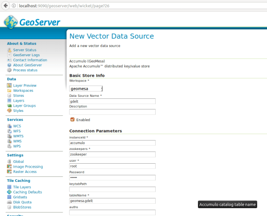
Then, we can create a new store of type Accumulo (GeoMesa) called “gdelt”. Use the following parameters:

instanceId = accumulo
zookeepers = zookeeper
user = root
password = GisPwd
tableName = geomesa.gdelt

Geodocker

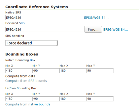
Then we can configure a Layer that publishes the content of our new data store. It is good to check the coordinate reference system settings and insert the bounding box information:

Geodocker2

To preview the WMS, go to GeoServer’s preview:

http://localhost:9090/geoserver/geomesa/wms?service=WMS&version=1.1.0&request=GetMap&layers=geomesa:gdelt&styles=&bbox=-180.0,-90.0,180.0,90.0&width=768&height=384&srs=EPSG:4326&format=application/openlayers&TIME=2017-07-10T00:00:00.000Z/2017-07-10T01:00:00.000Z#

Which will look something like this:

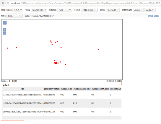
GeoMesa data filtered using CQL in GeoServer preview

For more display options, check the official GeoMesa tutorial.

If you check the preview URL more closely, you will notice that it specifies a time window:

&TIME=2017-07-10T00:00:00.000Z/2017-07-10T01:00:00.000Z

This is exactly where QGIS TimeManager could come in: Using TimeManager for WMS-T layers. Interoperatbility for the win!

Movement data in GIS #7: animated trajectories with TimeManager

By underdark

2017-08-14

Movement data in GIS, QGIS, Visualization

19 Comments

In this post, we use TimeManager to visualize the position of a moving object over time along a trajectory. This is another example of what is possible thanks to QGIS’ geometry generator feature. The result can look like this:

What makes this approach interesting is that the trajectory is stored in PostGIS as a LinestringM instead of storing individual trajectory points. So there is only one line feature loaded in QGIS:

(In part 2 of this series, we already saw how a geometry generator can be used to visualize speed along a trajectory.)

The layer is added to TimeManager using t_start and t_end attributes to define the trajectory’s temporal extent.

TimeManager exposes an animation_datetime() function which returns the current animation timestamp, that is, the timestamp that is also displayed in the TimeManager dock, as well as on the map (if we don’t explicitly disable this option).

Once TimeManager is set up, we can edit the line style to add a point marker to visualize the position of the moving object at the current animation timestamp. To do that, we interpolate the position along the trajectory segments. The first geometry generator expression splits the trajectory in its segments:

The second geometry generator expression interpolates the position on the segment that contains the current TimeManager animation time:

The WHEN statement compares the trajectory segment’s start and end times to the current TimeManager animation time. Afterwards, the line_interpolate_point function is used to draw the point marker at the correct position along the segment:

CASE 
WHEN (
m(end_point(geometry_n($geometry,@geometry_part_num)))
> second(age(animation_datetime(),to_datetime('1970-01-01 00:00')))
AND
m(start_point(geometry_n($geometry,@geometry_part_num)))
<= second(age(animation_datetime(),to_datetime('1970-01-01 00:00')))
)
THEN
line_interpolate_point( 
  geometry_n($geometry,@geometry_part_num),
  1.0 * (
    second(age(animation_datetime(),to_datetime('1970-01-01 00:00')))
	- m(start_point(geometry_n($geometry,@geometry_part_num)))
  ) / (
    m(end_point(geometry_n($geometry,@geometry_part_num)))
	- m(start_point(geometry_n($geometry,@geometry_part_num)))
  ) 
  * length(geometry_n($geometry,@geometry_part_num))
)
END

Here is the animation result for a part of the trajectory between 08:00 and 09:00:

This post is part of a series. Read more about movement data in GIS.